S. Hooman Hoseini1, S. Habib Musavi Jahromi2, M. Sadegh Rafi Vahid2
1Department of Civil engineering, Islamic Azad university of central Tehran branch, Tehran, Iran
2Department of Water engineering, Islamic Azad university of Tehran science and research, Tehran, Iran
Correspondence to: S. Hooman Hoseini, Department of Civil engineering, Islamic Azad university of central Tehran branch, Tehran, Iran.
| Email: |  |
Copyright © 2012 Scientific & Academic Publishing. All Rights Reserved.
Abstract
Side weirs are widely used in irrigation, land drainage, urban sewage systems, flood protection, and forebay pool of hydropower systems by flow diversion or intake devices. The hydraulic behavior of side weirs received considerable interest by many researchers. A large number of these studies are physical model tests of rectangular side weirs. In this study, Computational Fluid Dynamic (CFD) model together with laboratory model of rectangular broad-crested side weir were used for determining the discharge coefficient of the rectangular broad-crested side weir located on the trapezoidal channel. The discharges performances obtained from CFD analyses were compared with the observed results for various Froude number, Reynolds number and channel slope. The results obtained from both methods are in a good agreement. The average error between experimental and CFD Analyses is 5.13 %.
Keywords:
CFD, Laboratory Model, Rectangular Broad-Crested Side Weir, Discharge Coefficient
Cite this paper: S. Hooman Hoseini, S. Habib Musavi Jahromi, M. Sadegh Rafi Vahid, Determination of Discharge Coefficient of Rectangular Broad-Crested Side Weir in Trapezoidal Channel by CFD, International Journal of Hydraulic Engineering, Vol. 2 No. 4, 2013, pp. 64-70. doi: 10.5923/j.ijhe.20130204.02.
1. Introduction
Weirs are a small overflow-type dams commonly used to raise the level of a river or stream and cause a large change of water level behind them. It is likely that the flow discharge exceeds the capacity of a channel or river and, thus, a control structure such as side weirs should be employed to protect the system against overflow. Conventional side weirs are installed in the channel side wall, parallel to the flow direction and at a desired height so that when the water level rises to the weir height, some portion of flow would be deviated laterally. Occasionally, side weirs as a mean of water diversion can be used, as well.Nandesamoorthy et al.[17]. Subramanya et al.[22], Yu-tech[27], Ranga Raju et al.[19], Hager[11], Cheong[6], Singh et al.[21], Jalili et al.[13], and Borghei et al.[3] gave equations for discharge coefficients for rectangular, sharp-crested side weirs based on experimental results. Swamee et al.[23] used an elementary analysis approach to estimate the discharge coefficient in smooth side weirs through an elementary strip along the side weirs. Ghodsian [10] studied behavior in the rectangular side weir under conditions of supercritical flow. Yuksel[26] and Muslu et al.[16] used numerical analysis to analyze the flow over a rectangular side weir Recently, Aydin[2] modeled the free surface flow over the triangular labyrinth side weir by using Volume of Fluids (VOF) method to describe the surface characteristics in subcritical flow conditions. Borghei and Parvaneh[4] studied a new type of oblique side weir with asymmetric geometry on an experimental set-up. The researchers stated that this kind of weir is more efficient than the ordinary oblique weir. Emiroglu et al.[9] carried out a comprehensive study to determine the discharge coefficient of a sharp crested rectangular side weir in a straight channel, and developed an equation for discharge coefficient including all dimensional parameters. Agaccioglu et al.[1] presented a reliable equation based on 1504 experimental runs for discharge coefficient of the rectangular side weir in a curved channel depending on the all dimensionless parameters. Haddadi and Rahimpour[12] investigated an experimental setup to obtain the relationships of discharge coefficient with the other dimensionless parameters for trapezoidal broad-crested side weir. Bagheri S., Heidarpour [5] investigated the water flow over sharp-crested side weirs obtaining the distribution of the three- dimensional velocity.Considering the discharge dQ through an elementary strip of length ds along the side weir in a rectangular main channel in terms of De Marchi’s equation[8], one gets: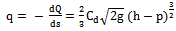 | (1) |
where Q is the discharge in the main channel, s is the distance from the beginning of the side weir, dQ/ds (or q) is the discharge overflow per unit length of the side weir, g is the acceleration due to gravity, p the is height of the side weir, h is the depth of flow at the section s (at s = 0 : h = h1 and Q = Q1), (h − p) is the pressure head on the weir and Cd is the discharge coefficient of the rectangular side weir. Thus, Qs = q.L, in which Qs is the flow rate over the side weir and L is the length of the side weir.Rafi Vahid[20] used Eq. (2) to estimate the discharge coefficient of broad-crested rectangular side weirs located in a trapezoidal channel, and he proposed the following equation for subcritical flow: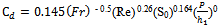 | (2) |
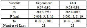
According to this point that no similar research has done yet in the rectangular broad-crested side weir located in the trapezoidal channel, and most of researches were conducted in the rectangular channel, therefore, this study presents a determination of discharge coefficient of the rectangular broad-crested side weir located in the trapezoidal channel in the subcritical flow condition by using CFD simulations with ANSYS FLUENT V.14, and the simulation results were compared with the experimental results.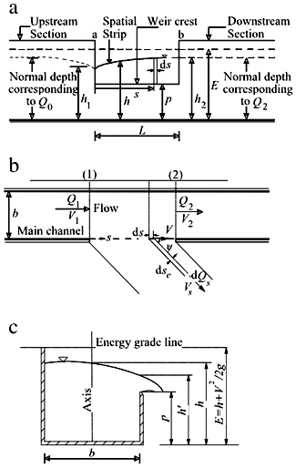 | Figure 1. Definition sketch of subcritical flow over a side weir.[9] |
 | Figure 2. Experimental arrangement |
2. Physical Model
The experiments were conducted at the Soil Conservation and Watershed Management Research Institute, Tehran, Iran. The data used in this study were taken from the experimental studies conducted by Rafi Vahid[20] on a large model. The experiments were carried out in a trapezoidal channel of internal width 1m, 30 m long and 0.88 m deep with a bed slope of zero and side slope 1:2 and bottom slope 0.001, 0.003. The side weir was located at a distance 13 m from the beginning of the main channel. The range of the various parameters is given in Table 1. For a given side weir, flow depth in the main channel was adjusted by a suitable sluice gate. Depth of flow in the main channel and the flow depths were measured at the centerline of the main channel, using a point gauge with an accuracy of 0.01 mm. The discharges in the main channel extension and the side weir were also measured by the volume method. Water for the main channel was supplied by pump and the flow was controlled by a gate valve 0.569 combinations were examined through various combinations of side width (b): 80 cm; side weir heights (P): 0.001, 5, 8, and 10 cm; side weir length (L): 4 m. A schematic representation of the experimental set-up is shown in Fig. 2.Table 1. Range of variables tested
 |
| |
|
3. CFD Model Description
ANSYS FLUENT V.14 is the CFD solver for choice for complex flow ranging from incompressible (transonic) to highly compressible (supersonic and hypersonic) flows. This paper represents a 3D modeling a flow over a rectangular broad-crested side weir in trapezoidal channel. In this study, used Second Order Upwind discretization scheme for Momentum, First order upwind discretization scheme for turbulent kinetic energy and turbulent dissipation rate; used Presto discretization scheme for Pressure and SIMPLEC algorithm for Pressure-Velocity Coupling Method. The under-relaxation factors are chosen between 0.2 and 0.5. The small values of the under-relaxation factors are required for the stability of the solution of this interpolation scheme. In the iterative solutions, it must be ensured that iterative convergence is achieved with at least three orders (1e-3) of magnitude decrease in the normalized residuals for each equation solved. For time dependent problems, iterative convergences at every time step are checked and all residuals are dropped below four orders (1e-4) in about 10,000 iterations. The time steps size are selected as t=0.1s.
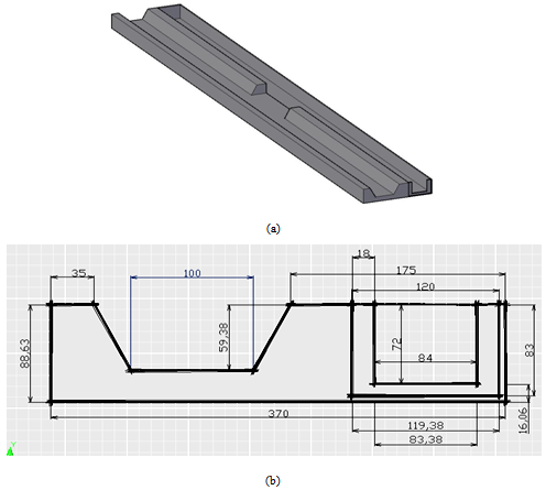
3.1. Geometry and Boundary Conditions
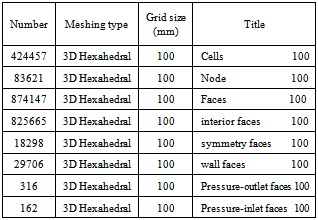
The geometries and meshes were generated by using ANSYS V.14. The parameters of the created models and its meshing pacifications were given in Table 2. The typical view of Geometry and mesh of model is given in Fig. 3. The open channel boundary conditions were applied to the CFD mode laste pressure inlet at the main channel inlet, the symmetry at the boundaries which open to atmosphere, the pressure outlet at the main channel outlet and secondary channel outlet, Also Wall boundary is used to specify the solid surfaces. The pressure inlet boundary condition presents an option which ensures to easily describe the bottom and the surface levels of the main channel and also the velocity of the main channel flow. A water level of downstream weir is imposed initially by the pressure inlet boundary at the main channel outlet. It is assumed that the free surface levels of the inlet and outlet boundaries in the main channel are approximately equal initially. After the solution is converged, the water levels reach own natural level in the subcritical conditions. For subcritical outlet flows (Fr< 1), if there are only two phases, then the pressure is taken from the pressure profile specified over the boundary, otherwise the pressure is taken from the neighboring cell. Based on the Froude number when Fr<1 the flow is known to be subcritical where disturbances can travel upstream as well as downstream. In this case, downstream conditions might affect the flow upstream[18].Table 2. Meshing specifications
 |
| |
|
 | Figure 3. Schematic view of mesh |
3.2. VOF Equation Discretization and Free Surface Reconstruction
The evolution of the volume fraction field F is governed by Eq. (3)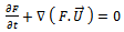 | (3) |
The upwind-biased characteristic method developed by Zhao et al.[28] is too diffusive for the evolution of step function. In this work, the CICSAM (Compressive Interface Capturing Scheme for Arbitrary Meshes) discussed in Lv et al.[15] is employed for its good performance to maintain the sharpness of the interface while keeping reasonable accuracy. It makes use of the NVD concept[14] and switches between different high resolution differencing schemes to yield a bounded scalar field, but one which preserves both the smoothness of the interface and its sharp definition (over one or two computational cells). The derivation of the scheme is based on the recognition that no diffusion of the interface (whether physical or numerical) can occur; thus it is only appropriate for sharp fluid interfaces. The scheme is based on the finite volume technique and is fully conservative. The special implicit implementation embedded inside makes it applicable to unstructured meshes. Interface reconstruction is the essential part of the coupled VOF method, i.e., given the interface normal vector in a cell, the unique linear interface segment (line segment in 2D and planar surface in 3D) which also truncates the cell by the given volume fraction must be found. Analytical relations connecting linear interfaces and volume fractions in triangular and tetrahedral grids have been presented in Yang et al.[25]. The merit of this method is that the analytic formulations eliminate the need for iteration, and thereby improve accuracy and reduce computation time. (The volume of fluid is exactly conserved during this form of interface reconstruction). After the planar interface in each free surface tetrahedron (defined by F ¼ 0:5) has been reconstructed analytically, the level set field needs to be re-distanced, which is also an essential step in normal level set method. This can be easily done for each grid point in the computational domain by finding the shortest distance to the reconstructed VOF interface, and an efficient lookup algorithm within the group of VOF planar interfaces is needed to save CPU time. For details on the implementation of the finite volume discretization of VOF equation and free surface reconstruction, the reader is referred to Lv et al.[15].
3.3. Modeling Turbulence Effects
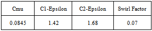
For the present computations, we use a renormalized group RNG  model due to the presence of highly strained regions in the flow and the irability to accurately predict moderate and low Reynolds number regimes[24]. In the case of the
 RNG model, a modification for including the local compressibility effects can be applied directly in the expression of the turbulent viscosity. The function
  , which is simply equal to ρ1 for a single phase flow, is turned to
 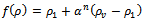 in the case of cavitating flows, with n=10.[7]. For modeling the flow close to the wall, standard wall function approach is used with enhanced wall functions approach applied in the near wall region. The range of y* values for which wall functions are suitable depend on the overall Reynolds number of the flow. The lower limit always lies in the order of y*~15. Below this limit, wall functions will typically deteriorate and the accuracy of the solutions cannot be maintained. The upper limit depends strongly on the Reynolds number. For very high Reynolds numbers (e.g., ships, airplanes), the logarithmic layer can extend to values as high as several thousand, whereas for low Reynolds number flows (e.g., turbine blades, etc.) the upper limit can be as small as 100. For these low Reynolds number flows, the entire boundary layer is frequently only of the order of a few hundred y* units. The application of wall functions for such flows should therefore be avoided as they limit the overall number of nodes one can sensibly place in the boundary layer. In general, it is more important to ensure that the boundary layer is covered with a sufficient number of (structured) cells than to ensure a certain y* value. In ANSYS FLUENT, the log-law is employed when y*>11.225. When the mesh is such that y*<11.225 at the wall-adjacent cells, ANSYS FLUENT applies the laminar stress-strain relationship that can be written as U*=y*. It should be noted that, in ANSYS FLUENT, the laws of the wall for mean velocity and temperature are based on the wall unit y* rather than y+. These quantities are approximately equal in equilibrium turbulent boundary layers. The parameters of the RNG k–ε model were given in Table 3.
Table 3. parameters of the RNG k–ε model
 |
| |
|
4. Results and Discussions
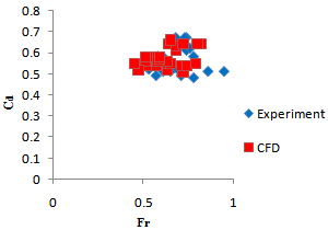 | Figure 4. Comparison of Cd coefficients against the Froude number |
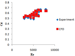 | Figure 5. Comparison of Cd coefficients against the Reynolds number |
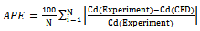
The discharge coefficients Cd of CFD models were calculated by Eq. (2) using the data obtained from CFD analyses as calculated by Rafi Vahid[20] for his physical model. Rafi Vahid[20] found that the discharge coefficient Cd for rectangular broad-crested side weir in trapezoidal channel depends on three dimensionless parameters: Froude number (Fr), Reynolds number (Re) and channel slope (S0). Therefore, in the CFD analyses, to show the effects of parameter Fr and Re on discharge coefficients, Cd values obtained from both the CFD and physical models are plotted against the dimensionless Froude number, Reynolds number and channel slope respectively in Figs. 4, 5 and 6. These figures show that Cd decreases with the increasing Fr and increases with the increasing Re and S0. Fig. 7 shows the comparison of Cd values obtained from CFD studies against the observed Cd. As it can be seen from Figs. 8, the discharge coefficients from CFD analyses are quietly compatible with the experimental data observed. In this Figure, the discharges coefficient obtained from CFD analyses and computed from Eq. (2) with Cd values obtained from experimental analyses by Rafi Vahid[20] were compared. As seen in this figure, the CFD and the experiment values are in reasonable agreement. Additionally, to evaluate the accuracy between experimental and CFD results, the root mean square error (RMSE) and the average percent error (APE) criteria were used. The RMSE and APE are given as 2.42 % and 5.13 % respectively for the side weir discharges for N=28. These values present a satisfactory agreement between experimental and CFD results.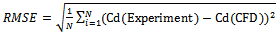 | (4) |
 | (5) |
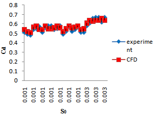 | Figure 6. Comparison of Cd coefficients against the channel slope |
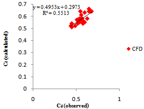 | Figure 7. Comparison of Observed and Calculated values of Cd |
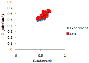 | Figure 6. Comparison of values of Cd obtained from CFD and Experimental analyses |
5. Conclusions
In the present study, the CFD (ANSYS FLUENT V.14 ) analyses of broad-crested side weir located on a trapezoidal channel were performed to investigate the effects of some dimensionless parameters as Fr, Re and S0 at the certain values of Cd. The open channel boundary conditions used in the CFD models provide an efficient approach for simulation of the flow over the rectangular broad-crested side weir. Both the results of CFD and physical model showed that while Cd coefficient decreases with increasing values of Fr and Cd coefficient increases with increasing values of Re. For all results, it is concluded that a reasonable agreement was achieved between the CFD results and the experimental observations. Additionally, an interval error of RMSE 2.42 % and APE 5.13 % respect to the side weir discharge coefficients between CFD and experimental results is reported. The presented results in this study can encourage further the researchers in making new different designs of rectangular side weir by using CFD.
List of symbols
References
| [1] | Agaccioglu H, Emiroglu ME, Kaya N. (2012). Discharge coefficient of side weirs in curved channels. Proceedings of the ICE–Water Management. 165 (WM6), 339–52. |
| [2] | Aydin MC. (2012). CFD simulation of free-surface flow over triangular labyrinth side weir. Advances in Engineering Software. 45, 159–66. |
| [3] | Borghei SM, Jalili MR, Ghodsian M. (1999). Discharge coefficient for sharp crested side weir in subcritical flow. J Hydraul Eng. 125(10), 1051–6. |
| [4] | Borghei SM, Parvaneh A. (2011). Discharge characteristics of a modified oblique side weir in subcriticalflow. Flow Measurement and Instrumentation. 22(5), 370–6. |
| [5] | Bagheri S, Heidarpour M. (2012). Characteristics of flow over rectangular sharpcrested side weirs. Journal of Irrigation and Drainage Engineering ASCE. 138(6), 541–7. |
| [6] | Cheong HF. (1991). Discharge coefficient of lateral diversion from trapezoidal channel. J Irrig Drain Eng. 117(4), 461–75. |
| [7] | Coutier-Delgosha, O., Fortes-patella, R., Reboud, J.L. (2003). Evaluation of the turbulence model: influence on the numerical simulations of unsteady cavitation. J. Fluids Eng. 125, 38–45. |
| [8] | De Marchi G. (1934). Saggio di teoria del funzionamento degli stramazzi laterali. Energ Elet. 11, 849–60 (in Italian). |
| [9] | Emiroglu ME, Agaccioglu H, Kaya N. (2011). Discharging capacity of rectangular side weirs in straight open channels. Flow Measurement and Instrumentation. 22(4), 319–30. |
| [10] | Ghodsian M. (2004). Flow over triangular side weir. Sci Iran. 11(1), 114–20. |
| [11] | Hager WH. (1987). Lateral outflow over side weirs. J of the Hydraul Division. 113(4), 491–504. |
| [12] | Haddadi H, Rahimpour M. (2012). A discharge coefficient for a trapezoidal broad-crested side weir in subcritical flow. Flow Measurement and Instrumentation. 26, 63–7. |
| [13] | Jalili MR, Borghei SM. (1996). Discussion of ‘Discharge coefficient of rectangular side weir, by ‘R. Singh, D. Manivannan and T. Satyanarayana’. ASCE Journal of Irrigation and Drainage Engineering. 122(2), 132. |
| [14] | Leonard BP. (1991). The ULTIMATE conservative difference scheme applied to unsteady one-dimensional advection. Comput Methods Appl Mech Eng. 88, 17–74. |
| [15] | Lv X, Zou QP, Reeve DE, Zhao Y. (2009). A novel coupled level set and volume of fluid method for sharp interface capturing on 3D tetrahedral grids. J Comput Phys. 229(7), 2573–604. |
| [16] | Muslu Y, Uyumaz. (1985). A Flow over side weirs in circular channels. Journal of the Hydraulics Division ASCE. 111(1), 144–60. |
| [17] | Nadesamoorthy T, Thomson A. (1972). Discussion of spatially varied flow over sideweirs. J Hydraul Eng. 98(12), 2234–5. |
| [18] | N.H. Lebanon. (2005). F.L.U.E.N.T. Inc. Fluent version 6.2 User’s Guide.: FLUENT Inc. |
| [19] | Ranga Raju KG, Prasad B, Gupta S. (1979).Side weir in rectangular channel. J of the Hydraul Division. 105(5), 547–54. |
| [20] | Rafi Vahid M.S. (2013). Experimental investigation of discharge coefficient for a Broad-Crested Side Weir in Trapezoidal Channel. Msc. thesis. Islamic Azad university of Tehran science and research, Tehran, Iran. |
| [21] | Singh R, Manivannan D, Satyanarayana T. (1994). Discharge coefficient of rectangular side weirs. J Irrig Drain Eng. 120(4), 814–9. |
| [22] | Subramanya K, Awasthy SC. (1972). Spatially varied flow over side weirs. J. of the Hydraul Division. 98(1), 1–10. |
| [23] | Swamee PK, Pathak SK, Ali MS. (1994). Side weir analysis using elementary discharge coefficient. J Irrig Drain Eng. 120(4), 742–55. |
| [24] | Yakhot, V., Orszag, S.A. (1986). Renormalization group analysis of turbulence. J. Sci. Comput. 1, 3–51. |
| [25] | Yang X, James A, Lowengrub J, Zheng X, Cristini V. (2006). An adaptive coupled levelset/ volume-of-fluid interface capturing method for unstructured triangular grids. J Comput Phys. 214, 41–54. |
| [26] | Yüksel E. (2004). Effect of specific variation on lateral overflows. Flow Measurement and Instrumentation. 15(5–6), 259–69. |
| [27] | Yu-Tek L. (1972). Discussion of spatially varied flow over side weir. ASCE J of the Hydraul Division. 98(11):2047–8. |
| [28] | Zhao Y, Tan HH, Zhang BL. (2002). A high-resolution characteristics-based implicit dual time-stepping VOF method for free surface flow simulation on unstructured grids. J Comput Phys. 183, 233–73. |
 Abstract
 Reference
 Full-Text PDF
 Full-text HTML