Briti Sundar Sil, Preetam Banerjee, Ajeet Kumar, P. Jarken Bui, Pallavi Saikia
Department Civil Engineering, Tezpur University, Tezpur, 784028, India
Correspondence to: Briti Sundar Sil, Department Civil Engineering, Tezpur University, Tezpur, 784028, India.
| Email: |  |
Copyright © 2012 Scientific & Academic Publishing. All Rights Reserved.
Abstract
In water supply system the function of carrying water is done through well planned distribution system choosing suitable diameter of pipes as it comprises the major investment in the system. Analysis and design of a pipe network system is a complex and time taking work. Now a day’s lot of pipe software is available which can be used suitably for layout and analysis of pipe network system. Working with professional software requires both money and training. Sometimes it is required to design a simple pipe network system for which an easy method will be suitable. In this paper a simple method is discussed which can be used suitably for optimal design of pipe networks for the water distribution system. The problem in this paper has thus been solved with a view to reduce the total cost of pipe network satisfying the required amount discharge in the outlet. Hardy Cross method has been used for estimating the required discharge in each outlet of the pipe network, and optimization of the system has been done to reduce the cost with the help of Microsoft-excel. The proposed optimization setup has been very close to the original value, thereby validating its use for optimization.
Keywords:
Solver, Pipe Network, Optimization, Water Distribution
Cite this paper: Briti Sundar Sil, Preetam Banerjee, Ajeet Kumar, P. Jarken Bui, Pallavi Saikia, Use of Excel-Solver as an Optimization Tool in Design of Pipe Network, International Journal of Hydraulic Engineering, Vol. 2 No. 4, 2013, pp. 59-63. doi: 10.5923/j.ijhe.20130204.01.
1. Introduction
In a water distribution system, water is supplied to consumers, through a series of system. Raw water collected from a reservoir is treated in a water treatment plant and make it suitable for drinking purpose which is then stored in an elevated water tank. From the tank, water is supplied in a controlled way to the consumer through a complex network system. This system for distributing water contains pipes, reservoirs, pumps, valves of different types, which are connected to each other to provide water to consumers. It is a vital component of the urban infrastructure and requires significant investment. The process of distributing water generally consists of different phases like proper layout for distributing system, designing of pipe network and process of operation, water treatment in the plant. The problem of optimal design of water distribution networks has various aspects to be considered such as hydraulics, reliability, material availability, water quality, and infrastructure and demand patterns.In water distribution system, the pipe layout is done as per the demand and available users. The objective here is to determine the optimal diameters of pipes in a network with a predetermined layout. This includes providing the pressure and quantity of the water required at every demand node. The problem of optimizing network requires the determination of pipe sizes from a set of commercially available diameters ensuring a feasible least cost solution. Here we have considered a two – loop network supplied by gravity with the objective of determining the minimum cost for a given layout. The cost of realizing the network is a function of the diameters. The smaller the diameter, the lower is the price. However the energy head at the consumers also decrease, therefore the problem is to minimize the cost under the constraint that the energy heads at the interior nodes are above some given lower limits.Discharge and pipe head losses are determined using Hardy Cross method satisfying the continuity equation. The algebraic sum of the pressure drops around a closed loop must be zero. This secures the overall mass balance in the network. For  number of nodes in the network, this can be written as
 | (1) |
Where  represents the total discharges in the
  node. The desired discharge value for the predetermined loop of the network system is optimized, considering the diameters of the pipes in the network as decision variables, the problems can be considered as a parameter optimization problem with dimension equal to the number of pipes in the network. Market constraints, however, dictate the use of commercially available pipe diameters. With this constraint the problem can be formulated in Microsoft Excel, where the optimization is done by Newton – Raphson Method.
2. Literature Review
As the pipe networking works involve a huge amount of money, so there have been many endeavors to optimize the pipe networks so that the cost gets lowered. Various methods of optimization have been developed, implemented and validated on many different pipe networks by many researchers so far. Most of the works of optimization have been applied on some standard water distribution networks like the Two-loop water distribution network ( first presented by Alperovits and Shamir)[1] consisting of 7 nodes, 8 pipes and two loops, fed by gravity from a reservoir with a 210 m fixed head. The scope of this work deals with the optimization of two loop pipe network presented by Alperovits and Shamir[1], so the various works carried out earlier on optimization of the said two-loop network has been discussed. The Work was further modified by Goulter et al.[2]. They also followed the LP method and the result was that the minimum cost they obtained was $ 435,015. Kessler and Shamir[3] further modified the work and obtained the results as $ 417,500. Both Goulter et al.[2] and Kessler and Shamir[3] used the LP approach and modified the work by optimizing the network by changing the pipe diameters.Fujiwara and Khang[4], Sherali and Smith[5] and Sherali et al.[6] further worked on the same two loop network presented by Alperovits and Shamir[1] and obtained their results as $ 415,271 , $ 436,684 and $ 436,915 respectively.Longanathan et al.[7] and Cunha and Sousa[8] used the Simulated annealing (SA) approach for optimization and thereby came to results of $ 412,931 and $ 419,000 respectively. Savic and Walters[9], Abebe and Solomatine[10] and Prasad and Park[11] took Genetic algorithm (GA) for optimization and obtained results of $ 419,000 each.Todini[12], Eusuff and Lansey[13] used Resilience Index, Harmonic Search (HS) and Shuffled frog leaping algorithm respectively for solution and obtained results of $ 419,000 each.In 2006, Z.W. Geem[14] applied a modified version of Harmony search method and obtained the cost as $ 419,000 in two loop network whereas the cost were found to be 0.28-10.26% less than those of competitive meta-heuristic algorithms, such as the genetic algorithm, simulated annealing etc. in other networks. In 2008, Onder et.al.[15] presented an optimization strategy based on head losses minimization is developed for the least cost design of water distribution networks. A new weighting approach was suggested for calculating the initial flow distribution and optimum pipe diameters of the weighted flow distribution was presented by using least square method. In the meantime homogenous and isotropous head losses are maintained with implications of head loss path choice. The model is employed for designing and modifying pipe sizes while the classical Hardy-Cross network solver is used to balance the flows. The whole algorithm is programmed and applied to a two-looped network selected from the literature and the results were presented on a comparative basis. A FORTRAN software with the necessary steps in the flow chart was written for the optimization calculations in his paper. With this minimum head loss strategy he obtained the cost as $ 416,000.In 2010, C.R.Suribabu[16] used Differential Evolution Algorithm (DEA)and arrived at the result of $ 419,000.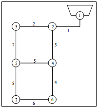 | Figure 1. Layout of two loop pipe network |
The two-loop network, shown in figure 1, was originally presented by Alperovits and Shamir[1]. The network has seven nodes and eight pipes with two loops, and is fed by gravity from a reservoir with a 210-m (=689 ft.) fixed head. The pipes are all 1000m (=3281 ft.) long with a Hazen-Williams coefficient C of 130. The minimum head limitation is 30m (=98.4 ft.) above ground level.
3. Objective of the Present Study
Objective of the present study is to provide a solution for optimization using Microsoft Excel solver tool. The objective here is to determine the optimal diameters of pipes in a network with a predetermined layout. This includes providing the water required at every demand node satisfying the minimum required conditions of pressure and discharge. The objective here, requires the determination of pipe sizes from a set of commercially available diameters ensuring a feasible least cost solution and that too without the involvement of such technical complexities which are present in most of the complex programs, algorithms and search mechanisms employed for optimization so far.
4. Methodology
In the present study, the two-loop network where flow occurs due to gravity is taken into account. It was first formulated using Linear Programming Gradient method by E. Alperovits and U. Shamir[1].The aim of the water distribution network analysis is to find least cost pipe network by optimizing pipe diameters in such a way that the analysis fulfills water demand and required pressure head in every node. To find out the optimal values, two modules, namely hydraulic module and an optimization module are brought into consideration. Both the process has been compiled using a solver application of excel spreadsheet.
4.1. Model Formulation
The model which has been formulated to accomplish the required task is done by formulating a hydraulic module which deals with the hydraulic aspects and the optimization module which deals with the optimization aspect and then compiling both the processes using a solver application in Microsoft excel spreadsheet. Flow chart of the model is shown in figure 2.
4.1.1. Hydraulic Module
The hydraulic module consists of hydraulics part where pipe flow analysis is done using Hardy-cross method.
4.1.2. Analysis of Pipe Network
For the analysis of pipe network, the following two necessary conditions must be satisfied.1. The algebraic sum of the pressure drops around a closed loop must be zero, i.e. there can be no discontinuity in pressure. 2. The flow entering a junction must be equal to the flow leaving the same junction; i.e. the law of continuity must be satisfied. Based upon these two basic principles, the pipe networks are solved by the method of successive approximation because any direct analytical solution is not possible. The analysis of a pipe network requires many equations, most of which being nonlinear, to be solved simultaneously.
4.1.3. Hardy-Cross Method
The procedure suggested by Hardy and Cross (Garg S.K,[17]) requires that the flow in each pipe be assumed by the designer (in magnitude as well as direction) in such a way that the principle of continuity is satisfied at each junction ( i.e. the inflow at any junction becomes equal to the outflow at that junction). Correction to these assumed flows is then computed successively for each pipe loop in the network, until the correction is reduced to an acceptable magnitude. If  is the assumed flow and
  is the actual flow in the pipe, then the correction
  is given by
 | (2) |
 | (3) |
Now expressing the head loss (HL) as | (4) |
where, (for Hazem-William formula)
 = length of pipe between two node.
 = a constant (1.852, for Hazen Williams formula ; 2, for Mannings or Darcy Weisbach formula)the head loss in a pipe can be calculated as
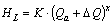
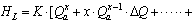 negligible terms of higher power
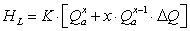 | (5) |
Now around a closed loop, the summation of head loss must be zero.i.e  Since
Since  is same for the all the pipes of the considered loop, it can be taken out of the summation.Therefore,
 | (6) |
Since  is given the same sign (or direction) in all pipes of the loop, the denominator of the above equation is taken as the absolute sum of the individual items in the summation. Hence
 | (7) |
 | (8) |
Where  = head loss for the assumed flow
  The numerator of the above equation is the algebraic sum of the head losses in the various pipes of the closed loop computed with the assumed flow. Since the direction and magnitude of flow in these pipes is already assumed, their respective head losses with due regard to sign (The head loss in clockwise direction may be taken as +ve and that in the anti-clockwise direction as -ve) can be easily calculated after assuming their diameters. The absolute sum of respective
  is then calculated. Finally the value of
  is found out for each loop, and the assumed flows in each pipe are corrected by using equation (8). Pipes common to two loops will receive both corrections with due attention to sign. After correcting the flows in the entire pipe network in the first iteration, the second correction can be applied to the already corrected flows in the previous step, and the re-corrected flows are again worked out in the entire network (consisting of one or more loops). The flows in pipes, common to two loops, should be corrected for the computed corrections of both the loops, as stated earlier. The procedure can be repeated to obtain more accurate results.The hydraulic module selects the optimal pipe sizes in the final network satisfying all constraints such as conservations of mass and energy and on the other hand pressure head and design constraints. The hydraulic constraints, for example, deal with hydraulic head at certain nodes to meet a specified minimum value. However, diameter constraints enforce the algorithms to select the trial solution within a predefined limit. A hydraulic network solver handles the implicit constraints and simultaneously evaluates the hydraulic performance of each trial solution that is a member of population of points. The hydraulic model first checks the head across each node of whether it satisfies the minimum pressure head conditions and then keeps on iterating until the minimum pressure head condition is satisfied by changing the diameter of each pipe within a given diameter range. Optimization module selects best fitted diameters from a set of diameters and minimizes the total cost of the pipe network.
4.1.4. Optimization Module
The optimization model involves the use of an excel solver which estimates the cost of the network and settles with the least cost satisfying all the constraints. The network cost is calculated as the sum of the pipe costs where pipe costs are expressed in terms of cost per unit length. Total network cost is computed as follows: | (9) |
where,  = cost per unit length of the
 pipe with diameter
  ,
, = length of the
  pipe.The optimization module keeps on checking the combination of pipe diameters satisfying the head conditions and resulting in the least cost of the network.While using solver for the optimization the following parameters was kept as constraints:(i) Pressure head across each node must be at least 30m.(ii) The diameter of the any of the pipe must be within the range of 0.025m-0.508m.
5. Model Applications
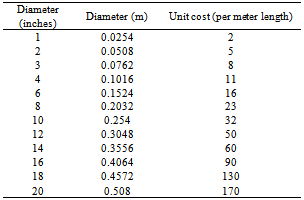
Table 1. Pipe diameters and their corresponding costs
 |
| |
|
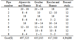
The application part involves the application of the two modules viz. the hydraulic module and the optimization module compiled using a solver application of excel spreadsheet onto the Two-loop pipe network proposed by Alperovits and Shamir. For finding the cost incurred, data provided in table 1 have been taken for pipe diameters available in the market and their unit costs per meter length.Then the optimization for least cost was carried out based on the above data in Microsoft Excel and the sizes of the respective pipes and the total cost incurred was determined which was compared with some earlier works and the results are shown in table 2.Table 2. Comparison of pipe diameters and total cost for two loop network
 |
| |
|
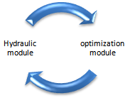 | Figure 2. Flow chart of the model |
6. Conclusions
The three basic components which consist of water distribution system are pumps, storage tanks and pipe networks. Optimization helps in reducing the cost of pipe networks by selecting and recognizing to adopt the best possible diameter to guarantee the best flow rate. The design for optimal distribution of the network is a complex task, A number of search methods, complex programs and algorithms have been proposed and attempted for the main concern of designing the most least cost network simultaneously satisfying the required minimum pressure head and discharge at the demand nodes. However, Microsoft Excel was used here for optimization to achieve the minimum cost but at the same time it also holds some drawbacks as it does not involve complex mechanisms for optimization as in the case of many algorithms which employ complex mechanisms for search of global optimal solution.As these methods involve complex algorithms, programs and function which require a lot of technical know-how’s it becomes difficult to implement such mechanisms for optimization by everyone in many cases. So our approach was to provide with an easy method for optimization which doesn’t involve such complexities.As is clear from the results embodied in this report, the cost incurred was lesser than that of Alperovits and Shamir; this is a good option for optimization if one doesn’t want to go into such complexities. The total cost however could have been a bit lower as well and well near about the range of some other works on the same network. But the reasons for such fluctuations might be because of the following reasons:1. As we have used Darcy Weisbach’s formula for determination of head loss and the value of n is assumed to be 2 for turbulent flows, whereas in many cases Hazen-William Equation has also been used and the value of n is taken near about 1.85, so this might be a cause for fluctuations in the total cost.2. Further another reason might be that we have assumed . For comparison and validation of the optimization method used in this paper, the application has been limited to two loop networks only. So there is a need to apply the same methodology for complex network also where more than two loops exist. Notations:
 = total cost
 = cost per unit length of the
 pipe with diameter
  ,
, ,= Diameter of the kth pipe
 = Head loss
  = Hazem-William
 = length of pipe between two node.
 = length of the
  pipe.
pipe. = Actual flow
  = Assumed flow
  = total discharges in the
  node.
node.  = correction
  = a constant (1.852, for Hazen Williams formula ; 2, for Mannings or Darcy Weisbach formula)
References
| [1] | Alperovits E., Shamir U. Design of optimal water distribution systems, Water Resources Research., 13(6), 885–900, 1977. |
| [2] | Goulter, I.C, B. M Lussier, and D.R. Morgan. Implications of head loss path choice in the optimization of water distribution network, Water Resources Research., 22(5), 819-822., 1986. |
| [3] | Kessler, A. & U. Shamir. Analysis of the linear programming gradient method for optimal design of water supply networks. Water Res. Research, 1 25(7), 1469-1480., 1989. |
| [4] | Fujiwara, O., Khang D. B. A two phase decomposition method for optimal design of looped water distribution networks. Water Resources Research. 26(4), 539-549, 1990. |
| [5] | Sherali, H. D., Smith, E. P. A Global Optimization Approach to a Water Distribution Network Design Problem. Journal of Global Optimization. Vol. 11, pp. 107-132, 1997. |
| [6] | Sherali, H. D., Totlani, R., Loganathan, G. V. Enhanced Lower Bounds for the Global Optimization of Water Distribution Networks. Water Resources Research. Vol. 34, No. 7, 1998. |
| [7] | Loganathan, G. V., Greene, J. J., and Ahn, T. J. Design Heuristic for Globally Minimum Cost Water-Distribution Systems. Journal of Water Resources Planning and Management, Vol. 121(2), 182-192, 1995. |
| [8] | Cunha, M.C. and Sousa, J. Water distribution network design optimization simulated annealing approach. Journal of Water Resources Planning & Management.125, 215 – 224., 1999. |
| [9] | Savic, D.A. & Walters G.A. Genetic algorithms for least-cost design of water distribution networks. WaterRes. Planning & Management, 123(2), 67-77., 1997. |
| [10] | Abebe, A.J. and Solomatine, D.P. Application of global optimization to the design of pipe networks. 3rd International Conferences on Hydroinformatics, Copenhagen, Denmark, pp. 989-996, 1998. |
| [11] | Prasad, T. D., and Park, N.S. Multiobjective genetic algorithms for design of water distribution networks. Journal of Water Resources Planning and Management, 130 (1), 73–82, 2004. |
| [12] | Todini, E. Looped water distribution networks design using a resilience index based heuristic approach. Urban Water, 2(2): 115–122., 2000. |
| [13] | Eusuff, M. and Lansey, K. Opimization of water distribution network design using the shuffled frog leaping algorithm. Journal of Water Resources Planning and Management, 129(3), 210-225, 2003. |
| [14] | Geem Z.W. Optimal cost design of water distribution networks using harmony search. Engineering Optimization Methods. , 38(3) , 259–280., April 2006. |
| [15] | Onder Ekinci and Haluk Konak. An Optimization Strategy for Water Distribution Networks. Water Resources Management. 23:169-185, 2009. |
| [16] | Suribabu C.R. Differential evolution algorithm for optimal design of water distribution networks, Journal ofHydroinformatics, 12.1,66-82, 2010. |
| [17] | Garg S.K. “Water Supply Engineering”, Environmental Engineering (Vol1), 733-735., 1977. |
 Abstract
 Reference
 Full-Text PDF
 Full-text HTML