-
Paper Information
- Previous Paper
- Paper Submission
-
Journal Information
- About This Journal
- Editorial Board
- Current Issue
- Archive
- Author Guidelines
- Contact Us
International Journal of Hydraulic Engineering
p-ISSN: 2169-9771 e-ISSN: 2169-9801
2013; 2(3): 53-58
doi:10.5923/j.ijhe.20130203.04
Numerical Representation of Weirs Using the Concept of Inverse Problems
 Abstract
 Reference
 Full-Text PDF
 Full-text HTML
Olesya I. Sarajlic1, Alexandra B. Smirnova2
1Department of Physics and Astronomy, Georgia State University, Atlanta, Georgia, 30303-3083, USA
2Department of Mathematics and Statistics, Georgia State University, Atlanta, Georgia, 30303-3083, USA
Correspondence to: Olesya I. Sarajlic, Department of Physics and Astronomy, Georgia State University, Atlanta, Georgia, 30303-3083, USA.
| Email: |  |
Copyright © 2012 Scientific & Academic Publishing. All Rights Reserved.
The use of Laplace transform and other computational tools allows the study of elementary inverse problems in hydraulics, such as for weirs. Torricelli's Law provides the relationship between the notch shape of the weir and the respective flow rate. The flow rate function r(h) gives the rate at which the volume of water hits the notch of a particular shape f(y). The essence of the direct problem here is to determine the flow rate r(h) from the notch shape f(y). Mathematically, this comes down to a computationally stable integration process. However, the corresponding inverse problem, i.e., identification of the notch shape f(y) from the flow rate measurements, is ill-posed in a sense that even a small error in the input data can result in a substantial inaccuracy in the computed solution. Numerical modelling offers the opportunity to test design parameters over large ranges and varieties of shapes. It may detect significant flow patterns and capture the amount of noise that a given function can tolerate. The goal of the study is to interpret the produced notch shape functions of the weirs, to discuss advantages and disadvantages of weirs' structure, and to present a regularized numerical algorithm for getting a less noisy and a more stable outcome of the inversion procedure.
Keywords: Weirs, Inverse Problems, Laplace Transform, Torricelli's Law, Lavrentiev’s Regularization
Cite this paper: Olesya I. Sarajlic, Alexandra B. Smirnova, Numerical Representation of Weirs Using the Concept of Inverse Problems, International Journal of Hydraulic Engineering, Vol. 2 No. 3, 2013, pp. 53-58. doi: 10.5923/j.ijhe.20130203.04.
Article Outline
1. Introduction
- Weirs are the overflow structures of defined shape that are built across open channels or streams to measure the flow rate[1-3]. There are several standard equations that are developed to describe the relations between the shape and design of the weir, rates of flow, head, and hydraulic conductivity[3]. Every design of the weir can be controlled by the depth of water, which in turn can predict how the crest elevation that is relative to the upstream head changes with discharge[4].There are two types of weirs, sharp-crested and broad-crested. Sharp crested weirs can take variety of shapes. The most common weir structures that are used for measuring irrigation water include rectangular, triangular (V-notch), trapezoidal (Cipolletti design), and parabolic weirs[4,5]. The designs of some weirs have certain advantages over the others. For example, the V-notch is designed to have small changes in discharge which results in a large change in depth of water through the notch allowing for a more accurate head measurement[6]. While V-notch weirs are built to monitor low flow conditions, Cipolletti weirs are designed to measure higher flows[1].There exist certain requirements to all sharp-crested weirs to assure accuracy of flow measurement. The most important ones are: the upstream face and head of the weir plates should be normal to the axis of the channel, the entire weir panel should have the same thickness, the edges of the weir opening should be straight and sharp, and other more technical conditions[4,7,8]. Once the weir is constructed, it can be tested and resulting calibrations can be compared with standard results. However, depending on the dimensions of the design, the weirs can cease to provide accurate measurements of the total stream flow during the events of prolonged heavy rainfall where the weirs are bypassed and the stream over-topped the banks[1].In the work that was done by Hively et.al.[1], the authors carried out the in-situ measurements of the range of flows through the V-notch and Cipolletti weirs, which dimensions were known. Unfortunately, several factors such as heavy rainfall, affected the accuracy of the measurements. In this work, the flow rate will be derived from the notch shape and vice versa. This method of computational analysis portends the outcome of the design, in particular Cipolletti and parabolic weirs, given the amount of relative error that can potentially disrupt the measurements.
2. Mathematical Background
- The principles of hydraulics serve as one of the branches of the fluid dynamics. Torricelli's theorem, which follows immediately from the law of conservation of energy, relates the velocity of the fluid flowing out of an elevated irrigation canal, fitted with a weir notch, under the force of gravity to the height of the water[9,10]. In what follows, we consider an elevated irrigation canal that is much wider in comparison to the weir notch; thus, there is an inconsequential change in water level when the sluice gate in the notch is removed. It is assumed that the weir notch is symmetric with respect to a central vertical axis so that for the non-negative values of x it can be characterized by the shape function x=f(y), see Figure 1.
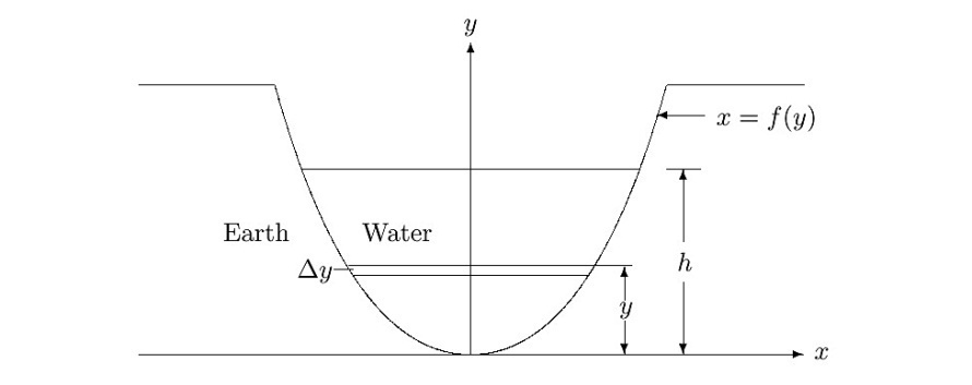 | Figure 1. A weir notch |
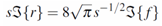
 | (1) |
 | (2) |
 | (3) |
3. Numerical Simulations: Weir Design
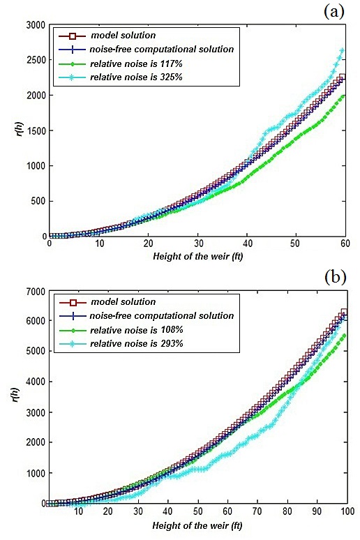
- Figure 2 shows the field constructed weirs that are typically used in agriculture with Figure 2(a) illustrating the Cipolletti design and Figure 2(b) being the parabolic weir. The shape functions for the Cipolletti and parabolic sharp-crested weirs are numerically fit to determine the corresponding flow rates by numerical integration carried out for equation (3).Figure 3 demonstrates stability of the direct problem where the Cipolletti weir with the shape function, f(y)
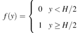 generates the flow rate r(h) of
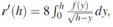
 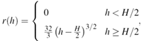 and H is the height of the weir. The original shape data f(y) is perturbed with random noise of various amplitudes to show the range of fault the computed flow rate r(h) can withstand before deviating from the model solution. Figure 3(a) illustrates the numerical simulation for the Cipolletti weir with height of 60 feet. As one can see, the model and the noise-free computed solutions of the direct problem are almost identical. If the shape data f(y) is perturbed with random noise of about 100%, which can be caused by the friction or the capillary effects of the water as it passes through the weir, the flow rate r(h) does not deviate from the exact solution significantly. Even when the relative noise increases to about 300%, the shape of the flow rate function can still be reconstructed. Figure 3(b) shows numerical outcomes for the Cipolletti shaped weir that is 100 feet high. The increase in noise levels produces similar results for the taller weir as for the shorter one. Hence the process of solving the direct problem is computationally stable, though the error in the computed flow rate does increase as the weir takes on higher value of height.The water flow through a parabolic sharp-crested weir can also be determined numerically by using equation (3). If the shape of the weir is defined as f(y)=√y, the corresponding solution for the flow rate that the weir is generating is r(h) = 2πh2. Figure 4 shows how stable the solution to the direct problem is even under a very high perturbation of the data. Similar to the case of Cipolletti weir, the noise-free computed flow rate for the parabolic weir notch has the same outcome as the model solution for both 60 and 100 feet inheight. Once a random noise higher than 100% or even 300% is added to the system, the flow rate can still be distinguished fairly easy, as Figure 4(a) and Figure 4(b) suggest. Analogous to the previous example, parabolic weir experiences great stability at short ranges of height. However, the flow function starts to deviate (slowly) from the model solution as the height becomes greater.
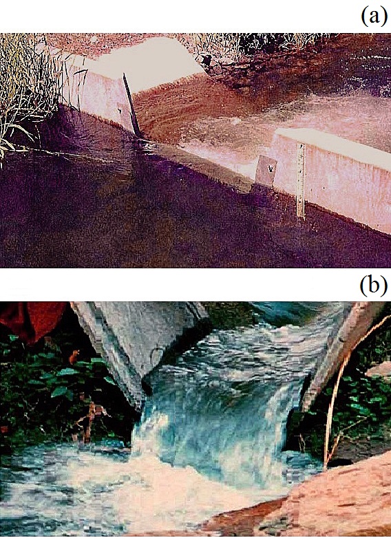 | Figure 2. Weir types - field constructed - that are commonly used in agriculture: (a) Cipolletti design that corresponds to the computational results in Figure 3, (b) parabolic weir corresponding to the numerical demonstration displayed in Figure 4 |
 and
and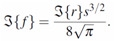 | (4) |

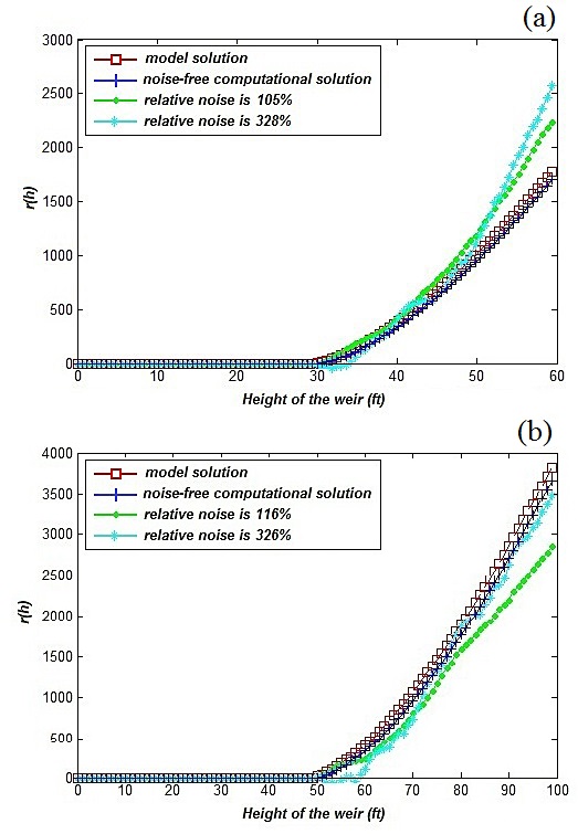 | Figure 3. Numerical demonstration of stability of the direct problem where the flow rate is 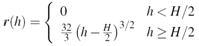 reconstructed from the shape reconstructed from the shape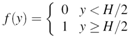 . Both exact shape data and shape data that is perturbed with random noise of various amplitudes were considered . Both exact shape data and shape data that is perturbed with random noise of various amplitudes were considered |
 and
and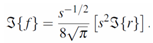 | (5) |
 | Figure 4. Numerical demonstration of stability of the direct problem where the flow function r(h)= 2πh2is reconstructed from the weir notch shape f(y)=√y. Both exact shape data and shape data that is perturbed with random noise of various amplitudes were considered |
 and, therefore, r´(0)=0. From the second equality in (5) along with the property r(0)=r´ (0)=0, one concludes
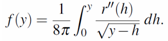 | (6) |
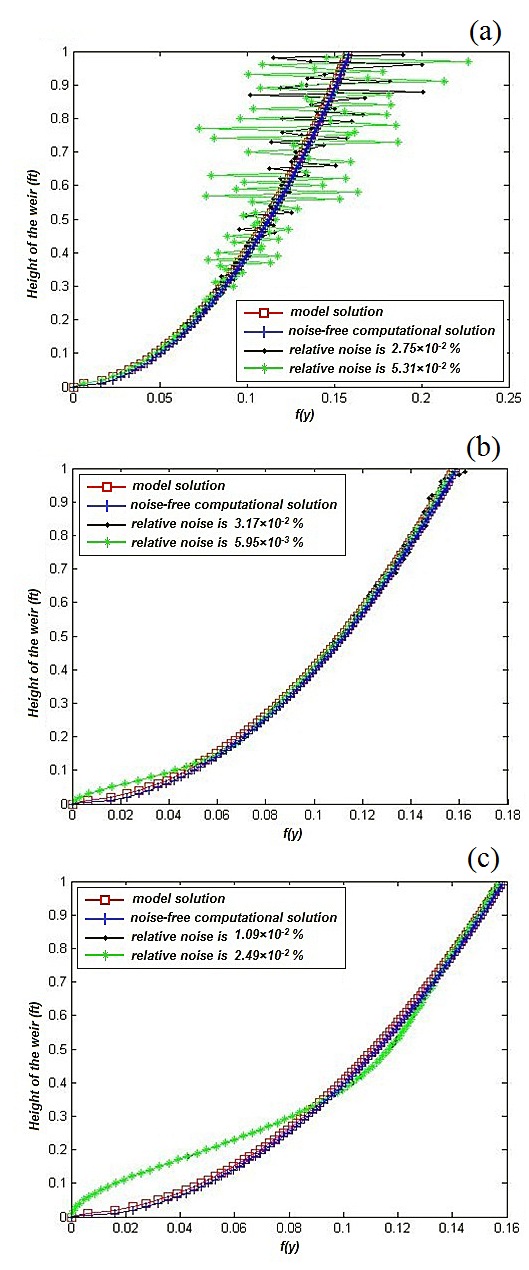 | Figure 5. (a) Illustrates f(y)= √y/(2π) reconstructed from r(h)=h2, cond(A)≈1050. (b) Illustrates f(y)= √y/(2π) reconstructed from r(h)=h2. Forα=0.1, cond(A+αI)≈69. (c) Illustrates f(y)= √y/(2π) reconstructed from r(h)=h2. Forα=0.5, cond(A+αI)≈16 |
4. Applications
- The design dimensions, specifications, placement locations, and other applications of various weir structures should be taken into consideration before the construction. The weirs were developed and subsequently applied to maintain the flow through the channel or stream in order to withstand floods, to protect stream banks from erosion by redirecting the flow, to enable sediment transport and deposition along the stream banks, to control flow direction in order to provide diversion of water for agricultural needs, and to maintain fish habitat and river stability[3,8].The numerical models of the parabolic weir (or Cross-Vane structure) and trapezoidal weir (Cipolletti design) that are illustrated on Figure 3 and Figure 4 can be manipulated to satisfy the requirements of the project before the actual construction. The Cross-Vane and Cipolletti structures have very beneficial aspects. Both Cross-Vane and Cipolletti weir designs can be used to maintain base level in the channels or streams and to reduce bank erosion by guiding the direction of the water flow to an angle orthogonal to the downstream weir face[3,8]. Another important aspect of parabolic and trapezoidal structures is the irrigation diversions. The structure is designed to create head differences at every point of the curve that enables the delivery of the water to the head gate at low flow rates. The construction of the sluice gate is considered as a part of the weir design in order to maintain the sediment delivery back to the channel which will reduce the relative error when deriving the expression for the flow rate from the notch shape function. Another application of the Cross-Vane with parabolic design is for the bridge and channel/stream stability. If there is a bridge constructed over the channel, then over time, high flow rates can cause bank erosion which can potentially occur at the support walls of the bridge. This problem can be reduced by construction a Cross-Vane in the upstream that will act as an offset[8].Although, the weirs are fairly beneficial and have variety of applications, their structures arelimited. There are maximum and minimum head, flow rate, angle, dimension restrictions that are considered to be standards when constructing a weir. The physical parameters restrain the use of the weirs in the channels or streams with extremely high flow rates, high heads, and/or wide areas of discharge.
5. Conclusions
- Several standard equations have been considered to describe the relations between the shape of the weir, rate of flow through a particular notch, head, and hydraulic conductivity. The use of Laplace transform, convolution theorem, and other computational tools allows the study of forward and inverse problems in irrigation theory. The flow rate r(h) can be determined from the notch shape f(y) through straightforward integration of equation (3), which is a very stable procedure and can withstand significant perturbation. On the other hand, the process of solving for the shape of the weir from known flow rate is unstable in a sense that even a small error in the input data can result in a substantial error in the computed solution. That is where the regularized numerical algorithm for getting a more stable product of the inverse problem comes into play. Thus, the method of computational analysis can predict the outcome of the constructed weir, in particular Cipolletti and parabolic weirs, given the amount of relative error that can potentially disrupt the measurements.
ACKNOWLEDGEMENTS
- We thank Seth Rose for helpful discussions on hydrogeological aspect of the paper. We would also like to acknowledge the use of the Visualization Wall facility at Georgia State University that is equipped with the Matlab software. This work was supported by National Science Foundation grant DMS-1112897.