S. K. Davletgaliev , L. K. Makhmudova
Department of meteorology and hydrology, Kazakh national university named after al-Farabi, Almaty, Kazakhstan
Correspondence to: S. K. Davletgaliev , Department of meteorology and hydrology, Kazakh national university named after al-Farabi, Almaty, Kazakhstan.
| Email: |  |
Copyright © 2012 Scientific & Academic Publishing. All Rights Reserved.
Abstract
Possibility group modeling of series annual amount of precipitations by a canonical expansion method is considered. Formulas and computer programs for statistical models of monthly and annual runoff of river are used. Model of canonical expansion preserves all statistical characteristics initial series.
Keywords:
Statistical Modeling, Canonical Expansion Method, Water Problems, Precipitation-runoff, Annual Precipitation, Statistical Parameters, Hydrologic Series, Modeling of Runoff
Cite this paper: S. K. Davletgaliev , L. K. Makhmudova , Statistical Modeling of Month and Annual Amount of Precipitations in Several Points Observations, International Journal of Hydraulic Engineering, Vol. 2 No. 1, 2013, pp. 14-19. doi: 10.5923/j.ijhe.20130201.02.
1. Introduction
When solving a number of water problems requires not only modeling of hydrological series, but series of precipitation. In particular, the modeling of runoff on the model of "rainfall-runoff", as well as in addressing a host of other practical problems need to know the different options for the onset of dry and wet periods in one and several observation points, so should be preserved type of distribution and the correlation structure of a number of observations. Canonical expansion model that meets these requirements and is used for modeling of hydrological series[1] can be used for statistical modeling of monthly precipitation. The effectiveness of modeling precipitation method canonical expansion compared to the models GM-2 and MM-1[2]. Here, the possibility of using the model for the canonical decomposition of artificial series of precipitation in several observation points[3].
2. Objectives and Methods
Getting multiple implementations monthly rainfall can be considered as the simulation of random vectors and processes defined in the end-time interval[4]. From this position, the best method for statistical modeling of precipitation is the method of the canonical decomposition. An important advantage of the method is its ability to model the enrichment related rainfall in several areas. The canonical decomposition of a vector random function in a natural way by the generalized formula-dimensional case[5]. For this, as shown in[6], is sufficient in appropriate proportions argument t replace all the arguments t and enter the number of components of the vector random function ℓ. Then the decomposition of a vector random function is given by the following formula: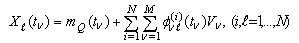 | (1) |
here, | (2) |
auto and cross-correlation function;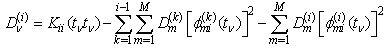 | (3) |
The variance of the random coefficients V;Kii (tν tμ) - correlation and cross-correlation function of the random vector function Xl (t); M - the number of intervals in the calculation year (months, decades)[.Here ν = 1,2,….M; μ > ν; μ= ν+1, ν+ 2,…M (at  =i); μ=1,2,…..M; l= i+1, i+ 2,…N (at
  >i).Equation (1) for the canonical decomposition of the three random functions of the form:
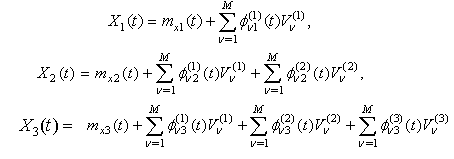 | (4) |
Where, mX1(t), mX2(t), mX3(t),-the expectation component X1(t), X2(t), X3(t); Vν(1), Vν(2), Vν(3) – uncorrelated random variables, expectations are zero;  – the mutual coordinate functions X(t) with constituents X2(t) и X3(t);
  – also make up X2(t) и X3(t);
  – the coordinate functions of the components X3(t).Statistical modeling of monthly rainfall is satisfied by (4). It follows that the first construct a canonical decomposition of the first component
  , as in the case of one-dimensional expansion, then the values
  ,
,  - the canonical decomposition second component
  , the functions
 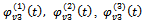 - the third component of the expansion
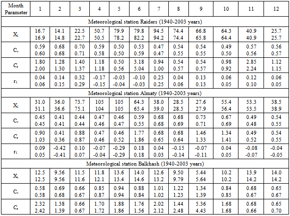
  [6]Monthly rainfall simulation time interval involves statistical analysis of data and the establishment of distribution law. Curve type of monthly precipitation can be installed in various ways. In this paper, as the basic law of the distribution used three-parameter gamma distribution Kritsky-Menkel. The main advantage of this distribution law is the possibility of its use for any relationships between the parameters Cv and Cs. As a measure of fit between the observed data and the theoretical curve of security used Pearson χ2 goodness of fit. At the same applied algorithm proposed in[7]. For each month is calculated coefficient Cv method of moments. Continue to consistently changing the ratio Cv/Cs from 1 to 6, according to the estimated degree of empirical and theoretical curves by χ2. The theoretical curve best fit the empirical material is chosen for the lower value of χ2. In Table 1 shown the results of calculation for the three points The data in Table 1 shows that at a significance level of 5 % and the number of degrees of freedom υ = 6 critical χ2 = 12,6 exceed one per meteorological station the Raiders and six cases per meteorological station the Balkhash. In this case, a significant discrepancy between the empirical data and the theoretical curve is observed in June (Rader city) and in April and September (Balkhash city). The results of calculations by χ2 is significantly affected by the presence of zero precipitation observations meteorological station the Balkhash. Analysis of these data by the Kolmogorov and nω2 showed good agreement of observations the three-parameter gamma distribution with the ratio Cv/Cs, shown in Table 1. So, for the June rainfall statistics λ = 0.80, nω2 = 0.061, for the April and September respectively precipitation received λ = 1.28, nω2 = 0.345 and λ = 1.28, nω2 = 0.260. These values are lower than the critical statistics λ5% = 1,36, nω25% = 0,4614. Therefore, we can assume that the precipitation of all the months and points approximately described by three-parameter gamma distribution. This is confirmed as being close empirical points about the theoretical curves security precipitation that month.Simulation algorithm month rainfall is as follows[8],[9]:1). Evaluation of homogeneity of observation series;2). Input data - implementation and monthly precipitation table K (P, Cv) for the distribution of S. Kritsky and M.F. Menkel in appropriate ratios of the parameters Cv and Cs.3). Computation of the expectations, the coefficients of variation and asymmetry of the correlation matrix of the moments and the normalized correlation matrix of autocorrelation coefficients of annual precipitation.4). Input relationship between parameters of the Cv and Cs.5). Unbiased assessment of the value of the coefficients of variation and autocorrelation.6). Determination of the amount of precipitation in the equation autoregressive based communication between adjacent members of the original series of precipitation.7). Calculation of the coordinate functions and the dispersion of random coefficients.8). Formation of the random coefficients Vv with a given standard deviation and mean zero.9). Realization of random variables in the equation of the canonical decomposition.10). Definition of probability (probability) variables computed in paragraph 9.11). Given that the three-parameter gamma distribution tables compiled for the fluidity of 0.001 to 99.9 %, the interval from 0 to 1, which is reproduced in the range of uniformly distributed, translated by a linear transformation to a new range - from 0.001 to 99.9 %.
Table 1. Assessment of compliance with a series of monthly rainfall distribution curve Kritsky-Menkel for various ratios Cv and Cs
 |
| |
|
12). Log on to the obtained values of security in the table of the distribution curve Kritsky-Menkel, for a given Cv and Cv/Cs and the calculation of the coefficients of modular precipitation by interpolation of the table values.13). A comparison of the statistical parameters of the original and simulated series.
3. Results
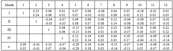
The results of calculations on the items revealed that three-dimensional model of the canonical decomposition is almost exactly reproduces the rules and coefficients of variation. Stability of the asymmetry coefficient is not sufficiently high. The convergence of this parameter with an initial value depends strongly on the length of the simulated series. When n = 3000 years, a considerable discrepancy (72.2 %) between the observed and modeled Cs series revealed in August (Balkhash city) at a high coefficient of variation Cv = 1.22. In other cases, the discrepancy between the values of Cs is not more than 20 %[10].The values of the first order autocorrelation coefficients r1 small. only for some months. their value reaches - 0.42 and + 0.32. In most cases the relationship of monthly precipitation adjacent years can be considered insignificant and monthly precipitation of the paragraphs independent random variables. Compliance with both positive and negative values of the autocorrelation coefficients to the raw data is quite satisfactory. Table 3 and 4 shows the (1). the formula can be used to simulate the annual precipitation at several points of observation. In this case. the equation of the canonical decomposition of random variables[2]. which for «n»-th number of points observations of precipitation is written as: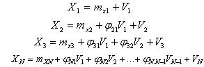 | (5) |
Where, N - number of meteorological station; - the expectation of random variables;х1, х2,...хn, V1, V2, …Vn - uncorrelated random variables, expectations are zero;φjk - factors that determine the conditions of uncorrelated variables V1, V2, …Vn.
Table 2. Statistical parameters of the average monthly amount of precipitation for the observed (1st line) and simulated (2nd line)
 |
| |
|
Table 3. Row-correlation matrix of monthly precipitation for the observed (1st line) and simulated (2nd line) Meteorological station Raiders (Leninogorsk) (n = 3000)
 |
| |
|
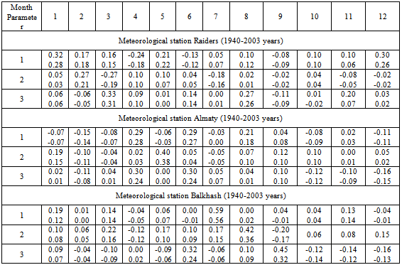
Table 4. Cross-correlation matrix of average monthly precipitation amount for the observed (1st line) and simulated (2nd line) of the series (n = 3000)
 |
| |
|
For simulation of annual precipitation by equation (1) we need to determine the values Di φjk, called the coordinate functions[11] and the variance of the random variables dl Vi. They can be determined from the following recurrence formulas[12]: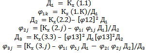 | (6) |
 for j for j = i. φij = 1.Values Di and φij calculated one after another in the order in which they appear in the calculations[2]. You need to know the correlation matrix of moments Кх(i.j). which defines it according to the available number of observations of the annual precipitation. Random variables Vi is formed in the standard program of the normal distribution.Simulation of annual precipitation involves statistical analysis of data and the establishment of distribution law. Curve type of rainfall can be installed in various ways. In this paper. as the basic law of the distribution used three-parameter gamma distribution Kritsky-Menkel. The main advantage of this distribution law is the possibility of its use for any relationships between the parameters Cv and Cs. The relation between the parameters Cv/Cs selected by χ2. It was found that the annual rainfall of all items considered satisfactorily described by Cs = 2Cv.Simulation algorithm of annual precipitation is little different from simulation algorithm runoff.φij coordinate functions and variance of random variables dl Vv calculated by the equations given in[13].That the method of canonical expansions for simultaneous simulation of the annual precipitation in several observation points is shown in the example of the 12 meteorological point of the Ural-Caspian basin.
Table 5. The statistical parameters of annual precipitation for the observed and (1st line) and simulated (2nd line) of the series (n = 1000)
 |
| |
|
Table 6. Cross-correlation matrix of annual precipitation for the observed and (1st line) and simulated (2nd line) of the series (n = 1000)
 |
| |
|
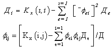
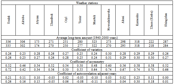
For a description of the annual precipitation in the region also adopted a three-parameter gamma distribution Kritsky-Menkel. The relation between the parameters Cv/Cs selected, as above, by χ2. It was found that the annual rainfall of all items considered satisfactorily described by Cs = 2Cv.Tables 5 and 6 show the statistical parameters of the observed annual precipitation (1940-2000 years) And simulated (n = 1000) of the series. Table 1 shows, the near coincidence of the rules and the coefficients of variation in the volume of the simulated sequence of n = 1000.Asymmetry coefficients simulated series are compared with the specified value Cs so ratio Cs/Cv set when choosing the law of distribution of annual precipitation. For individual points difference between the coefficients of asymmetry can be significant, but it is within the specified accuracy of calculation of Cs. The same conclusion can be drawn when considering the autocorrelation coefficients of adjacent years.The data in Table 6 show that the extent to which the cross-correlation coefficients given and obtained series can be considered quite high.
4. Conclusions
Thus, the series of precipitation simulated by the canonical decomposition, have statistical parameters close to the parameters of the observed series and keeps auto-and cross-correlation observed in the original series. Consequently, the method of expanding successfully will use for simultaneous modeling of annual precipitation in a few points of observation. This may be used by the algorithm and the calculation program, made to simulate river flow.
References
| [1] | I.V. Busalaev, S.K. Davletgaliev, I.G. Cooperman. Application of the method of canonical expansions for modeling river runoff // Problems of Hydropower and Water Management. Issue 10 p. 143-152, Almaty: Nauka, Kazakhstan, 1973. |
| [2] | Lee Suntak. A stochastic model to simulate the series of monthly amounts of precipitation and runoff values // Proceedings of International Symposium "Specific aspects of the hydrological calculations for the design of the water" Gidrometeoizdat, UNESCO Press, p. 382-393. USSR. 1981. |
| [3] | S.K. Davletgaliev. Joint modeling of the series of annual runoff by the canonical decomposition // Meteorology and Hydrology, № 10, pp. 102-108, Almaty, Kazakhstan, 1991. |
| [4] | V.G. Salnikov, G.K. Turulina, S.E. Polyakova, M.M. Moldakhmetov L.K. Makhmudova Fluctuations of the general circulation of the atmosphere, precipitation and runoff over the territory of Kazakhstan // Bulletin of the Kazakh National University, Series geographical. Number 1. pp. 23-27. Almaty, Kazakhstan. 2011. |
| [5] | S.N. Kritsky, M.F. Menkel. The methods of investigation of random fluctuations of river runoff. - Proceedings of the NIU GUGMS, Ser. 4. Issue 29, USSR. 1946. p. 3-32. |
| [6] | V.S. Pugachev. The theory of random functions. Physics and mathematical publishing, p. 884. USSR. 1962. |
| [7] | S.K. Davletgaliev, D.K. Dzhusupbekov, M.M. Moldakhmetov Mathematical processing of hydrological information. “Kazak universiteti” Publishing. p. 100. Almaty, Kazakhstan. 2012. |
| [8] | A.V. Rozhdestvensky, A.I. Chebotarev. Statistical methods in hydrology. Gidrometeoizdat, p. 415 USSR. 1974. |
| [9] | S.K. Davletgaliev. Statistical modeling of month and annual amount of precipitations in several points observations // Meteorology and Hydrology, № 10. p. 16-23. Russia. 2012. |
| [10] | M.M. Moldakhmetov, L.K. Makhmudova Estimation norm of annual runoff in the absence of a number of observations on the territory of the Republic of Kazakhstan // Bulletin Treasury Series geographical, Almaty. Number 2. pp. 76-79. Kazakhstan, 2010. |
| [11] | Davletgaliev S.K. Effects of management on the annual flow of the main rivers Zhaiyk Caspian Basin // Problems of Geography and Geoecology. № 1, pp. 4-11. Almaty, Kazakhstan. 2011. |
| [12] | M.M. Moldakhmetov, L.K. Makhmudova, A.K. Musina Assessment of the accuracy parameters of annual runoff in rivers Esil and Nura // Proceedings of the Fourth International Scientific Conference "Earth Sciences at the present stage." 24-25 April 2012, Moscow. pp. 421-427. Russia. 2012. |
| [13] | R.I. Galperin, M.M. Moldakhmetov, L.K. Makhmudova A.G. Chigrinets and A. Avezova Water resources of Kazakhstan: Evaluation, prognosis, management. Monograph Volume VII. Resources runoff Kazakhstan. Book 1. Renewable surface water resources of the West, North, Central Kazakhstan. LLP "Institute of Geography». p. 665. Almaty, Kazakhstan. 2012. |
 Abstract
 Reference
 Full-Text PDF
 Full-text HTML