-
Paper Information
- Next Paper
- Paper Submission
-
Journal Information
- About This Journal
- Editorial Board
- Current Issue
- Archive
- Author Guidelines
- Contact Us
International Journal of Hydraulic Engineering
p-ISSN: 2169-9771 e-ISSN: 2169-9801
2012; 1(6): 55-67
doi: 10.5923/j.ijhe.20120106.01
Comparing the Performance of Neural Networks for Predicting Peak Outflow from Breached Embankments when Back Propagation Algorithms Meet Evolutionary Algorithms
 Abstract
 Reference
 Full-Text PDF
 Full-Text HTML
Farhad Hooshyaripor, Ahmad Tahershamsi
Faculty of Civil and Environment Engineering, Amirkabir University of Technology, Tehran, Iran
Correspondence to: Ahmad Tahershamsi, Faculty of Civil and Environment Engineering, Amirkabir University of Technology, Tehran, Iran.
| Email: |  |
Copyright © 2012 Scientific & Academic Publishing. All Rights Reserved.
This investigation provides a review of some methods for estimation of peak outflow from breached dams and presents an effective and efficient model for predicting peak outflow based on artificial neural network (ANN). For this reason the case study data on peak outflow discharge were compiled from various sources and reanalyzed using the ANN technique to see if better predictions are possible. By employing two important effective parameters namely, height (Hw) and volume (Vw) of water behind the dam at failure, four scenarios were addressed. To train the models two different algorithms were examined namely, back propagation (BP) and imperialist competitive algorithm (ICA). Among the BP algorithms, Levenberg–Marquardt (LM), resilient back propagation (RP), fletcher–reeves update (CGF), and scaled conjugate gradient (SCG) were utilized. Therefore, 20 different ANN models were developed and compared to each other. Results showed that both Hw and Vw parameters are similarly dominant in estimating the peak outflow discharge. Among the different training functions, LM was the best, because of higher coefficient of determination (R2=0.87) and lower error (RMSE=9616). Comparing the results of ANN and empirical formulas indicated higher ANN performance, so such formulas are better to be replaced with superior ANN model.
Keywords: Dam Breach, Peak Outflow Discharge, Neural Network, Training Algorithm
Cite this paper: Farhad Hooshyaripor, Ahmad Tahershamsi, "Comparing the Performance of Neural Networks for Predicting Peak Outflow from Breached Embankments when Back Propagation Algorithms Meet Evolutionary Algorithms", International Journal of Hydraulic Engineering, Vol. 1 No. 6, 2012, pp. 55-67. doi: 10.5923/j.ijhe.20120106.01.
Article Outline
1. Introduction
- Dam failure is a catastrophic phenomenon that can lead to large damages to human life and property. Overviewing of historical dam failures shows that overtopping and piping were the major causes of dam failures. Overtopping is mostly dangerous for embankment dams because it washes away or erodes very quickly the dam’s materials. In Piping, water seeps under the dam and gradually erodes the dam materials. The extension of this phenomenon may lead to dam collapse. The various modes of breach formation in embankment dams, and the large number of factors that influence the outflow characteristics, are difficult to describe with rigorously precise mathematical formulas. Because of complexity and uncertainty resulting from the wide range of values of the effective parameters, it is worthwhile to reduce the mathematical complexity of the problem and to present simple methods to predict the outflow characteristics from breached embankment. Prediction of peak outflow is very important because of the emergency action plan preparation and risk assessment. In some former investigations, case study data were used to develop empirical formula by relating peak outflow to the height of water behind the dam and/or volume of water behind the dam. Some investigators developed single-variable equations[13],[21],[36-38],[42], and some others presented multi-variable equations[10], [16],[30],[31],[44]. Hagen[17] introduced “dam factor” as the product of height of water and reservoir storage volume at the time of failure, and proposed a formula relating the peak-breach outflow to the dam factor. Some investigators applied the dam factor in their proposed equations[11],[25].Although applying empirical equations based on statistical regression is simple in practice, they are unable to estimate the values of peak outflow accurately. It is felt that this is partly due to the complexity of the phenomenon involved and low accuracy of data driven from historical dam failures[14], and partly because of the limitation of the analytical tool commonly used by most of the earlier investigators namely, traditional statistical regression. Nowadays, traditional statistical analysis has been replaced by newly alternative approaches in many cases. Artificial neural networks (ANN) as an alternative approach have advantages over statistical models like their data-driven nature, model–free form of predictions, and tolerance to data errors[4]. ANN beside its simplicity and generalizing ability has been used widely in hydraulic[3],[5],[7],[24],[40],[41], [45]. Most of the studies have been done by feed forward back propagation (BP) neural network. The standard back propagation algorithm (SBPA) as the training algorithm in BP has some problems including the low training convergence speed and easy entrapment in a local minimum [19]. During last decades, researchers have tried to overcome these problems and improve the ANN performance. Ramirez et al.[32] proposed the resilient back propagation (RP) training function for network training to predict the rainfall in Sao Paulo, Brazil. According to their findings, using RP could improve the results. Some other researchers proposed Levenberg–Marquardt algorithm (LMA). Noori et al.[28] evaluated different training functions on ANN operation for predicting the monthly stream flow and found that fletcher – reeves update (CGF) and scaled conjugate gradient (SCG) models had the best performance in wet and arid periods, respectively. Chau[9] used particle swarm optimization to optimize the network weights and biases for predicting water level in Shing Mun River. He compared the results with the SBPA results and showed the superiority of his model. Rogers et al.[33] proposed genetic algorithm (GA) instead of SBPA. Accordingly, the objective of this study is to compile previously presented case study data on peak outflow discharge from breached embankments, and reanalyze the resulting database using the technique of neural networks with a view towards seeing if better predictions are possible. Hereby, different training functions consisted of RP, CGF, SCG, and LMA are examined. Besides, a new evolutionary algorithm, imperialist competitive algorithm (ICA), proposed by Atashpaz-Gargari and Lucas[1] is used to optimize the network weights and biases. Finally, the results are compared to result of empirical formulas.
2. Material and Methods
2.1. Data Collection And Empirical Formulas
- Valuable documented information is available from historical embankment failures. Babb and Mermel[6] summarized over 600 dam incidents throughout the world; however, high quality and detailed information was lacking in most cases. Here the data from 93 embankment dam failures (Table 1) are collected from variety of sources[15], [16],[30],[35],[39],[43],[44]. During the decades, several researchers compiled some data of well-documented case studies in efforts to develop predictive relations for breach peak outflows. Among them, Kirkpatrick[21] proposed a formula based on analysis of data from 13 failed embankment dams and 6 hypothetical failures:
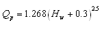 | (1) |
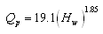 | (2) |
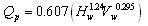
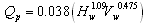
- Singh and Snorrason[37] used some simulated dam failures and presented Eq. (3):
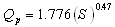 | (3) |
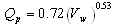 | (4) |
 | (5) |
 | (6) |
 | (7) |
 | (8) |
2.2. Neural Network Models
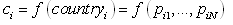
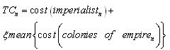
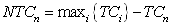
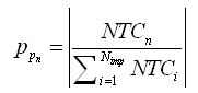
- An ANN is a ‘black box’ approach which has great capacity in predictive modeling[22]. It is a proper mathematical structure having an inter-connected assembly of simple processing elements or nodes. A typical network would consist of three layers of neurons namely, input, hidden, and output; in which each neuron acting as an independent computational element. Neural networks are universal approximators[20], and many theoretical and experimental works have shown that a single hidden layer is sufficient for ANNs to approximate any complex nonlinear function[12],[27],[29]. Accordingly, in this study single hidden layer ANNs were used. The tangent-sigmoid and linear functions were chosen as the activation function respectively in the hidden and output layers, and mean square error (MSE) was utilized as performance function. To check the over-fitting problem in the calibration and testing steps, stop training algorithm method was used. There are different training functions to optimize the network weights and biases in the case of BP algorithm. They can be divided into two different categories; the first one uses heuristic techniques, while the second one uses standard numerical optimization techniques. On the other hand, some other algorithms are available which use evolutionary optimization techniques (e.g. ICA) for training the network. Some details of ICA are available in the literatures[1,2]. The quick review of the above algorithms is as follow:Heuristic techniquesHeuristic techniques were developed from an analysis of the performance of the standard steepest descent algorithm. Gradient descent, gradient descent with momentum, gradient descent which has variable learning rate, gradient descent with momentum which has variable learning rate and RP are the most famous training functions which use heuristic techniques to update the network parameters. Because of using sigmoid transfer function in the hidden layer of multi-layer ANN with BP algorithm, the performance of the above training functions except RP can be affected[28]. So, in this research just RP is evaluated among the heuristic techniques.Standard numerical optimization techniquesThe SBPA adjusts the weights in the steepest descent direction (negative of the gradient) which the performance function is decreasing most rapidly. Although it decreases most rapidly along the negative of the gradient, this does not necessarily produce the fastest convergence. Conjugate gradient algorithms (CGA) are one of the fastest optimization techniques. In the CGAs for faster convergence than steepest descent directions a search is performed along conjugate directions. All the CGAs start out by searching in the steepest descent direction on the first iteration[28]. Discussion of CGAs and their application in neural networks are available in Hagan and Demuth[18]. The CGAs require that a line search be performed. Charalambous method, which was worked out in the present research, is a hybrid search which was designed to be used in combination with a CGA for neural network training. It uses a cubic interpolation together with a type of sectioning[8]. Various algorithms for CGA are available, e.g. CGF, SCG, Polak – Ribiere updates (CGP), and Powell–Beale restarts (CGB). Comparison of these algorithms on ANN operation for predicting the monthly stream flow has been done by Noori et al.[28]. Results indicated that the CGF and SCG were the best algorithms with superior performance, so they are employed in the present study.LMA developed by Levenberg[23] and Marquardt[26] is another type of standard numerical optimization techniques. LMA provides a numerical solution to the problem of minimizing a nonlinear function over a space of parameters of the function. These minimization problems arise especially in least squares curve fitting and nonlinear programming. LMA interpolates between the Gauss – Newton algorithm (GNA) and the method of gradient descent. LMA is more robust than GNA, which means that in many cases it finds a solution even if it starts very far off the final minimum. LMA is a very popular curve-fitting algorithm used in many software applications for solving generic curve-fitting problems; however, it finds only a local minimum, not a global minimum.Imperialist competitive algorithm ICA is a new evolutionary algorithm in the evolutionary computation field based on the human's socio-political evolution. The algorithm starts with an initial random population called countries. Some of the best countries in the population be selected as the imperialists and the rest form the colonies of these imperialists. In an N dimensional optimization problem, a country is a 1 × N array. This array is defined as below:
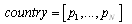 | (9) |
 | (10) |
 | (11) |
 | (12) |
 | (13) |
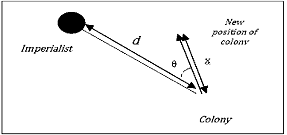 | Figure 1. Moving colonies toward their imperialist |
 | (14) |
 | (15) |
 | (16) |
 | (17) |
 | (18) |
3. Results and Discussion
- To evaluate different models, a database containing of 93 field and experimental dataset was used (Table 1). Out of the total input–output pairs, 85% were used for calibration (training and validation) and the remaining 15% were saved for testing. Since it was needed that the testing data be used for evaluating the empirical formulas, these data were chosen randomly from the category which had not been used in derivation of those formulas. Among the Eqs. 1 to 8, some take Hw as the independent variable (Eqs. 1 and 2), some take Vw as the independent variable (Eqs. 3 and 4), some take the dam factor as the independent variable (Eqs. 5 and 6), and the others take both of Hw and Vw as the independent variables (Eqs. 7 and 8). Accordingly, four scenarios were defined here and four sets of ANNs were developed in which the input variables were different. Furthermore, in order to evaluate the various training algorithms in each scenario, RP, CGF, SCG, LMA, and ICA were examined. So, totally 20 models were developed and compared to each other. To evaluate and compare the results, three statistical measures were utilized namely, coefficient of determination (R2); mean absolute error (MAE); and root mean square error (RMSE). For confidently evaluating the results, each modeling procedure, including calibration and testing steps, was iterated 50 times and the average values of the statistical measures were calculated. Therefore the expected values of the statistical measures were presented in this research.
3.1. First scenario’s Results (Considering Hw as the Input Variable)
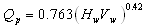
- In the first scenario it was assumed that peak outflow discharge (Qp) just relates to Hw. Table 2 shows the quantitative results of the ANN models as well as the empirical formulas. According to the results, all ANN models have moderate R2 value and high error. The RMSE for LMA is 14405 in testing step, which shows a high error. The error measures values in Table 2 show a different performance in training and testing steps e.g. the MAE values in testing steps are almost 3 times more than training step’s values. This ratio for RMSE values is almost equal to 2. Such results may be due to the below reasons:1. The Hw parameter can’t be sufficient for a model to predict the peak outflow discharge, lonely. In other words, some other parameters are important in peak discharge prediction and consequently the models developed based on just Hw has low efficiency. 2. The datasets are insufficient, so lower training may be happened; however, lack of datasets is a general problem in ANN application. It is clear that the more data available, the more accuracy in ANN modeling. 3. The method of data derivation in the field or laboratory has been inaccurate, and consequently some inaccurate data in the database may have been led to such error. Scale effects in experimental researches as well as estimation of peak outflow discharge from water-mark and stage-discharge curves in the field may be the main sources of error in recording the data. Fig. 2 presents the schematic performance of ANN model with ICA training function as the best model compared with observed values for both calibration and testing steps. As most of the values of peak outflow in training and testing step aren’t estimated correctly, the model performance isn’t satisfactory. Besides, as can be seen in Table 2, the Kirkpatrick and USBR formulas have a weak performance. The coefficient of determination for Kirkpatrick formula is very low (near 0.76) and its RMSE is 11732 which shows very high error. The situation is a little better for USBR formula but it is not satisfactory too because of low R2 (=0.74) and high error (RMSE =10656).
| |||||||||||||||||||||||||||||||||||||||||||||||||||||||||||||||||||||||
3.2. Second Scenario’s Results (Considering Vw as the Input Variable)
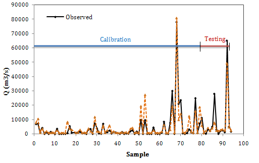
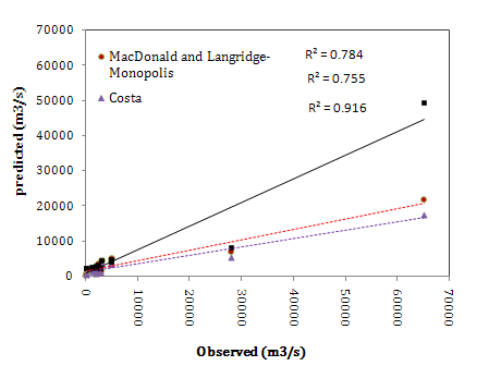
- In the second scenario the same database was used for training and testing steps, but the simulation was done with Vw instead of Hw as the input variable. The quantitative results are presented in Table 3. The coefficient of determination of each ANN model is good in both steps but the error measures are relatively high. Among the models RP has the highest RMSE value in the testing step and SCG has the lowest one. In this scenario although ICA has a good R2 value in testing step, it can’t be effective because of different R2 values in training and testing steps as well as high RMSE value. According to Table 3, it can be inferred that SCG has the best performance. The R2 values of Singh and Snorrason and Evans formulas respectively are 0.78 and 0.79, which means moderate performance compared to SCG. Fig. 4 shows the performance of ANN model compared to observed values. Although the results are some better than the first scenario, there are some points that aren’t predicted satisfactorily. Fig. 5 shows the ANN performance compared to empirical formulas. It is obvious that all the models underestimate the observed values especially extreme values. However the situation for SCG is much better, but not satisfactory.
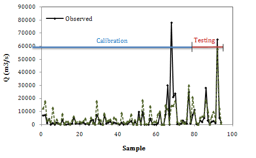 | Figure 2. Results of the best ANN model (ICA) in the first scenario |
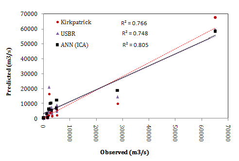 | Figure 3. Comparing the ANN results (ICA model) with empirical formulas results in the first scenario |
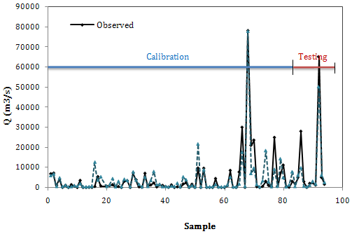 | Figure 4. Results of the best ANN model (SCG) in the second scenario |
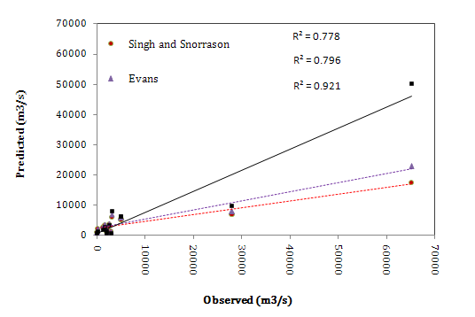 | Figure 5. Comparing the ANN results (SCG model) with empirical formulas results in the second scenario |
- By comparing Tables 2 and 3, it is found that R2 and error values for different models in the second scenario are more satisfactory. Therefore the models based on Vw parameter may lead to more reliable results due to extensive range of Vw parameter in dam breach database (3700 - 600106 m3).
3.3. Third Scenario’S Results (Considering Dam Factor as the Input Variable)
- In the third scenario, dam factor was employed in ANN modeling. Results of the best ANN model is presented in Fig. 6. It is observed that the predicted values are not so good. In some points the prediction values are about two times over than the observed values. The quantitive results are prepared in Table 4. In this scenario ICA has high R2 value and low RMSE in testing, so the ICA can be a good model but not exactly an effective model due to difference between the model performance in training and testing steps. Fig. 6 shows the results of ICA in calibration and testing steps.
 | Figure 6. Results of ANN model (ICA) in the third scenario |
 | Figure 7. Comparing the ANN results (ICA model) with empirical formulas results in the third scenario |
3.4. Fourth Scenario’s Results (Considering Hw and Vw as the Input Variables)
- In the last scenario both variables (Hw and Vw) are independently used in the ANN modelling. The quantitive results are presented in Table 5. As the results show, all the ANN models could predict peak outflow values very well because of high coefficient of determinations (R2> 0.80). Comparing the results indicates that MAE and RMSE values of ICA model are lower and its R2 value is higher than the other models’ in both training and testing steps. Fig. 8 shows ANN model performance in calibration and testing steps separately. It is clear that the model have a good so that most of the predictions are approximately coincided with their corresponding observed values. As it is illustrated in Fig. 8, there are approximately 5 points in the testing step and one point in the testing step which aren’t predicted satisfactorily. Like to the previous scenarios, most of the badly predicted points are corresponding to extreme values (large dams). Accordingly, one can strongly conclude that insufficient data or lack of historical data of large breached embankments is the main reason of lower training of the network.
| |||||||||||||||||||||||||||||||||||||||||||||||||||||||||||||||||||||||
| |||||||||||||||||||||||||||||||||||||||||||||||||||||||||||||||||||||||
| ||||||||||||||||||||||||||||||||||||||||||||||||
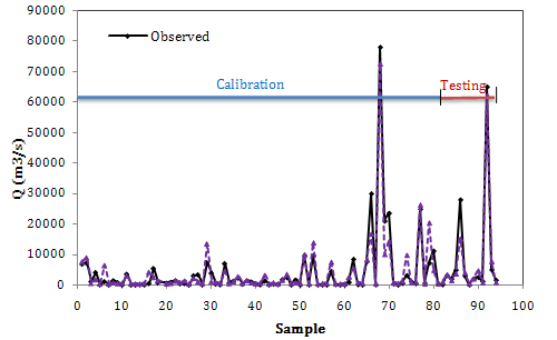 | Figure 8. Results of the best ANN model (ICA) in the fourth scenario |
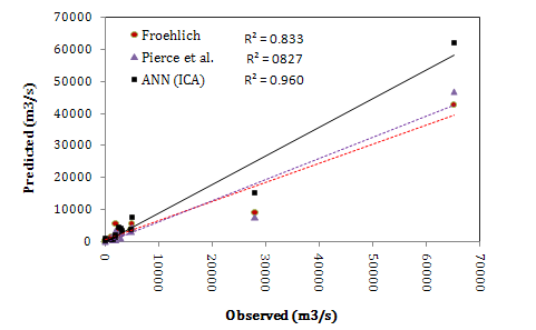 | Figure 9. Comparing the ANN results (ICA model) with empirical formulas results in the fourth scenario |
4. Conclusions
- This investigation focused on evaluating the ANN performance for predicting peak outflow from breached embankment dams. In order to find an effective model, four scenarios were defined. In scenarios I and II, it was assumed that Qp related respectively to Hw and Vw. In scenario III it was assumed that Qp related to the dam factor, and in scenario IV it was assumed that Qp related to the both Hw and Vw. Also to train the network, two training algorithms were employed: ICA and BP. ICA is a new evolutionary algorithm, in the evolutionary computation field, and BP algorithm is a common method of teaching ANNs called multi-stage dynamic system optimization method. By considering the statistic indices as well as CPU time taken, ICA was recognized as the best training algorithm in most of the scenarios. However, ICA takes a little more CPU time taken in comparison with the other algorithms. Also among the different scenarios, scenario IV was the best. In the scenarios I to III all ANN models underestimate the real extreme values, because the values related to large dam cases (i.e. Hw>15 m and/or Vw>50 mcm) are limited, so ANNs have not effectively been calibrated around the extreme values. Accordingly, enlarging the database by adding the values of new breached large dam cases or generating the synthetic extreme data may be effective. Moreover, results showed that the effect of Hw and Vw on the amount of peak outflow discharge was the same. This investigation indicated that although empirical formulas were simply applicable in practice, they lead to unsatisfactory results due to low R2 value and high error in their estimation especially for large breached dams. This is because of limited databases which were used in the formulas derivation as well as the low flexibility of the traditional method of regression analysis to data variation.
References
| [1] | E. Atashpaz-Gargari, and C. Lucas, “Imperialist competitive algorithm: An algorithm for optimization inspired by imperialistic competition”, IEEE Congress on Evolutionary Computation, pp. 4661–4667, 2007. |
| [2] | E. Atashpaz-Gargari, F. Hashemzadeh, R. Rajabioun, and C. Lucas, “Colonial competitive algorithm, a novel approach for PID controller design in MIMO distillation column process”, International Journal of Intelligent Computing and Cybernetics, vol.1, no.3, pp. 337–355, 2008. |
| [3] | F. Avarideh, M.A. Banyhabib, and A. Taher-shamsi, “Application of artificial neural networks in river Sediment estimation”, 3th Iran Hydraulic Conference, Kerman, Iran, pp. 269-275, 2001. |
| [4] | H.Md. Azmatullah, M.C. Deo, and P.B. Deolalikar, “Neural networks for estimation of scour downstream of a ski-jump bucket”, J. Hydraul. Eng., vol.131, no.10, pp. 898–908, 2005. |
| [5] | H.Md. Azamathulla, and A. Ghani, “ANFIS-based approach for Predicting the scour depth at culvert outlets”, Journal of Pipeline Systems Engineering and Practice, vol.2, no.1, pp. 35-40, 2011. |
| [6] | A.O. Babb, and T.W. Mermel, “Catalog of Dam Disaster, Failures and Accidents”, Bureau of Reclamation, Washington, Denver, Colo., 1968. |
| [7] | S.M. Bateni, and D.S. Jeng, “Estimation of pile group scour using adaptive neuro-fuzzy approach”, Ocean Engineering, vol.34, no.8-9, pp. 1344–1354, 2006. |
| [8] | C. Charalambous, “Conjugate gradient algorithm for efficient training of artificial neural networks”, IEEE Proceedings, vol.139, no.3, pp. 301–310, 1992. |
| [9] | K.W. Chau, “Particle swarm optimization training algorithm for ANNs in stage prediction of Shing Mun River”, J. Hydrol., vol.329, no.3-4, pp. 363-367, 2006. |
| [10] | S. Coleman, D. Andrews, and M.G. Webby, “Overtopping breaching of noncohesive homogeneous embankments”, J. Hydraul. Eng., vol.128, no.9, pp. 829–838, 2002. |
| [11] | J.E. Costa, “Floods from dam failures”, U.S. Geological Survey, Denver, 54, Open-File Rep. No. 85-560, 1985. |
| [12] | G. Cybenko, “Approximation by superposition of a sigmoidal function”, Math. Cont. Sig. Syst., vol.2, no.4, pp. 303-314, 1989. |
| [13] | S.G. Evans, “The maximum discharge of outburst floods caused by the breaching of man-made and natural dams”, Can. Geotech. J., vol.23, no.4, pp. 385–387, 1986. |
| [14] | D.L. Fread, “Some limitations of dam-break flood routing models”, Preprint, American Society of Civil Engineers, Fall Convention, St. Louis, Mo., October, 1981. |
| [15] | D.C. Froehlich, “Embankment dam breach parameters revisited”, Water Resources Engineering, Proc. 1995 ASCE Conf. on Water Resources Engineering, New York, pp.887 – 891, 1995a. |
| [16] | D.C. Froehlich, “Peak outflow from breached embankment dam”, J. Water Resour. Plann. Manage., vol.121, no.1, pp. 90–97, 1995b. |
| [17] | V.K. Hagen, “Re-evaluation of design floods and dam safety”, Proc., 14th Congress of Int. Commission on Large Dams, Rio De Janeiro, Brazil, vol.1, pp.475-491, 1982. |
| [18] | M.T. Hagan, and H. Demuth, “Neural Networks Design”, Boston, MA: PWS Publishing, 11.1-12.52, 1996. |
| [19] | S. Haykin, “Neural Networks: A ComprehensiveFoundation”, 2nd Ed., Prentice-Hall, Upper Saddle River, N.J, 1994. |
| [20] | K. Hornik, M. Stinchcombe, and H. White, “Multilayer feedforward networks are universal approximators”, Neural networks, vol.2, no.5, pp. 359-366,1989. |
| [21] | G.W. Kirkpatrick, “Evaluation guidelines for spillway adequacy”, The evaluation of dam safety, Engineering Foundation Conf., ASCE, New York, pp.395–414, 1977. |
| [22] | S. Lek, and J.F. Guegan, „Artificial neural networks as a tool in ecological modelling, an introduction“, Ecol. Model., vol.120, no.2-3, pp.65-73,1999. |
| [23] | K. Levenberg, “A method for the solution of certain non - linear problems in least squares”, Quart. Appl. Math, vol.2, no.2, pp.164–168,1944. |
| [24] | S.L. Liriano, and R.A. Day, “Prediction of scour depth at culvert outlets using neural networks”, J. Hydroinformatics, vol.3, no.4, pp.231–238, 2001. |
| [25] | T.C. MacDonald, and J. Langridge-Monopolis, “Breaching characteristics of dam failures”, J. Hydraul. Eng., vol.110, no.5, pp.567–586, 1984. |
| [26] | D.W. Marquardt, “An algorithm for least-squares estimation of nonlinear parameters”, J. Soc. Ind. Appl. Math., vol.11, no.2, pp.431–441, 1963. |
| [27] | R. Noori, M.A. Abdoli, A. Farokhnia, and M. Abbasi, “Results uncertainty of solid waste generation forecasting by hybrid of wavelet transform-ANFIS and wavelet transform - neural network”, Expert Systems with Applications, Vol.36, pp.9991–9999, 2009. |
| [28] | R. Noori, M.S. Sabahi, and A.R. Karbassi, “Evaluation of PCA and Gamma test techniques on ANN operation for weekly solid waste predicting”, J. Environ. Manage., vol.91, no.3, pp.767-771,2010. |
| [29] | R. Noori, A.R. Karbassi, H. Mehdizadeh, and M.S. Sabahi, “A framework development for predicting the longitudinal dispersion coefficient in natural streams using artificial neural network”, Environ. Prog. Sustain. Energ., vol.30, no.3, pp.439-449,2011. |
| [30] | M.W. Pierce, C.I. Thornton, and S.R. Abt, “Predicting peak outflow from breached embankment dams”, J. Hydrol. Eng., vol.15, no.5, pp.338–349, 2010. |
| [31] | M. Pilotti, M. Tomirotti, G. Valerio, and B. Bacchi, “Simplified method for the characterization of the hydrograph following a sudden partial dam break”, J. Hydraul. Eng., vol.136, no.10, pp.693–704, 2010. |
| [32] | M.C.V. Ramirez, N.J. Ferreira, and H.F. Velho, “Artificial neural network technique for rainfall forecasting applied to the Sa˜o Paulo region”, J. Hydrol., vol.301, no.1-4, pp.146 – 162, 2005. |
| [33] | L.L. Rogers, F.U. Dowla, and V.M. Johnson, “Optimal field-scale groundwater remediation using neural networks and the genetic algorithm”, Environ. Sci. Techno., vol.29, no.5, pp.1145–1155,1995. |
| [34] | H. Sepehri Rad, and C. Lucas, “Application of imperialistic competition algorithm in recommender systems”, 13th Int. CSI Computer Conference (CSICC'08), Kish Island, Iran, 2008. |
| [35] | V.P. Singh, and P.D. Scarlatos, “Analysis of gradual earth dam failure”, J. Hydraul. Eng., vol.114, no.1, pp.21–42,1988. |
| [36] | K.P. Singh, and A. Snorrason, “Sensitivity of outflow peaks and flood stages to the selection of dam breach parameters and simulation models”, State Water Survey (SWS) Contract, Illinois Dept. of Energy and Natural Resources, SWS Div., Surface Water at the Univ. of Illinois, Rep. no.288,1982. |
| [37] | K.P. Singh, and A. Snorrason, “Sensitivity of outflow peaks and flood stages to the selection of dam breach parameters and simulation models”, J. Hydrol., vol.68, pp.295–310, 1984. |
| [38] | Soil Conservation Service, “Simplified Dam-Breach Routing Procedure”, Technical Release, No.66 (Rev.1), 39p, December 1981. |
| [39] | A. Taher-shamsi, A. V. Shetty, and V. M. Ponce, “Embankment Dam Breaching: Geometry and Peak Outflow Characteristics”, Dam Engineering, vol.14, no.2, pp.73-87, 2004. |
| [40] | A. Taher-shamsi, M.B. Menhaj, and R. Ahmadian, “Sediment loads prediction using multilayer feedforward neural networks”, Amirkabir Journal of Science and Technology, vol.16, no.63, pp.103-110, 2006. |
| [41] | R. Trent, N. Gagarin, and J. Rhodes, “Estimating pier scour with artificial neural networks”, Proc., Stream Stability and Scour at Highway Bridges, E. V. Richardson, ed., ASCE, Reston, Va., pp.171–171,1999. |
| [42] | U.S. Bureau of Reclamation, “Guidelines for defining inundated areas downstream from bureau of reclamation dams”, Reclamation Planning Instruction, no. 82-11,1982. |
| [43] | T.L. Wahl, “Prediction of embankment dam breach parameters”, A literature review and needs assessment, Bureau of Reclamation, U.S. Department of the Interior, Denver, 60, Rep. no. DSO-98-004, 1998. |
| [44] | Y. Xu, and L.M. Zhang, “Breaching parameters for earth and rockfill dams”, J. Geotech. Geoenviron. Eng., vol.135, no.12, pp.1957-1970,2009. |
| [45] | M. Zounemat-Kermani, A. Beheshti, B. Ataie-Ashtiani, and S. Sabbagh-Yazdi, “Estimation of current-induced scour depth around pile groups using neural network and adaptive neuro-fuzzy inference system”, Appl. Soft Comput., vol.9, no.2, pp.746–755,2009. |