1. Introduction

Computational Fluid Dynamics (CFD) models have found widespread use in ecohydraulic assessments[1-4]. One of the most important aspects of using CFD for this purpose is to capture flow field complexity. Eddies and velocity gradients that result from interaction between flow and channel roughness such as large rocks and woody debris are important because invertebrates utilize such environments[5-7]. In general, flow and habitat complexity resulting from the occurrence of large roughness elements and habitat quality may be positively correlated[8].

As demonstrated by Crowder and Diplas[2], field data of rivers often captures only the bathymetry while omitting the large scale roughness elements. CFD models typically account for this omission by applying a global roughness value across a large area of the channel. This simplification however, clearly diminishes the local influence of individual rocks and thus mitigates the effective utility of the model for the purposes of ecological assessments. This limitation has been addressed by explicitly representing individual large rocks within the CFD[3,4,9]. Explicit modeling of large woody debris (LWD), on the other hand, has been much more limited. This is not surprising given that detailed field measurement of complex large woody debris and the subsequent computational mesh development can be very difficult. Inadequate meshing practices can leave cells highly distorted, causing numerical diffusion, solution instability, and convergence issues[10].

LWD can be a significant source of form drag in a river and can account for 50 percent of the total drag in the channel[11]. LWD plays an important role in stream morphology and is often introduced into streams at reach and watershed scales as part of restoration actions. Given the difficulty in modeling LWD with CFD, it is likely that the hydraulic effects and subsequent linkages to the ecology are not well represented in most CFD models.

Previous experimental studies involving turbulent obstructed flow in river systems include the examination of obstructed flow surrounding various boulder profiles[12]. Although these authors naturally encountered local flow variations, they did find similar flow patterns within the turbulent wake of each boulder. They used the results to further discuss how these related to natural channel design and fish habitat. Lacey and Roy[13] also incorporated acoustic velocimetry to characterize turbulent flow around various large roughness elements. They further utilized multivariate regression analysis as a tool to better predict wake turbulence.

Complementary to the experimental studies, numerical simulations can also offer an additional means for analyzing turbulent obstructed flow from LWD’s. Unlike the experimental studies mentioned previously, however, a comparable quantity of numerical LWD simulations is severely lacking. While several numerical investigations of turbulent flow in natural stream settings attempt to account for the effects of sediment[14-21], these are generally limited to fairly small grain size distributions. The effects of these flow obstructions are often accounted for by the incorporation of a roughness length. Several field studies have related the total roughness length (k_s) to a particle diameter at a certain percentile of the grain size distribution of natural streams[22]. However, there are substantial limitations to utilizing large roughness lengths that may affect the accuracy and stability of solutions. Additionally, most reliable roughness models restrict the roughness length to one-half the near-bed cell thickness[23]. This can become impractical for beds composed of cobbles or even gravels because of the constraints on the amount of flow detail that can be resolved in streams with larger grain sizes. Solution stability and solution accuracy become problematic. If larger near-bed cells are utilized, the cell centroid may no longer fall within the law of the wall region[24]. Modeling LWD’s utilizing roughness length representations remains therefore unfeasible.

In natural settings, most LWD boundaries are highly complex and non-uniform. In such cases it is often impractical to model their complex surfaces without using an excessive number of grid elements. Insufficient grid resolution can lead to the near-boundary cells being highly distorted, causing numerical diffusion, solution instabilities, and convergence problems. As a result, relatively few studies have attempted to address the effects of individual flow field obstructions, such as large woody debris[25]. Those that do exist are, in general, conducted using idealized simplifications of the actual geometries that they wish to represent[12]. These geometric simplifications, for example, will often include idealized spheres and cylinders to represent boulders and logs, respectively. The localized and downstream effects of these simplifications on the surrounding flow field when contrasted with non-idealized cases are not well understood. These uncertainties may also be contributing to imprecise conclusions concerning the quality, preservation, and growth of fish habitat in and around these structures.

Based on these uncertainties, the objective of this work is to quantify the numerical effect of LWD geometric simplification on the surrounding flow field. Specifically, the local velocity and turbulent kinetic energy will be numerically computed for each of three successively refined LWD geometries. Turbulence modeling will be accomplished via the unsteady Reynolds-averaged Navier-Stokes (URANS), utilizing one of three selected turbulence closer models. For each geometry, a shape complexity factor is computed and used to quantify a relative means for comparison. Preliminary validation, specifically relating to the choice of turbulence closure model, will be first examined through the use of a simplified 3D benchmark study, conducted experimentally by Lyn and Rodi[26] and Lyn et al.[27].

2. Validation Method

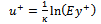
For model validation purposes, the physical experiments performed by Lyn and Rodi[26] and Lyn et al.[27], corresponding to the high Reynolds number, 3D turbulent flow of water over a square cylinder, were selected. This particular application was selected due to its relevance to unsteady viscous flow characteristics behind bluff bodies at high Reynolds’ numbers. Additionally, the study has served as a benchmark for the validation of several different turbulence closure models, including those of DNS, LES and RANS related studies[28-30].

One of the most challenging problems associated with turbulence modeling is the accurate prediction of boundary layer flow separation from solid surfaces. While Large Eddy Simulation (LES), has in recent years assumed the primary role in the simulation of these types of flows, a growing number of URANS based turbulence closure models have also shown significant promise. Compared to LES, RANS based models, particularly linear two equation models, although inherently less accurate, are attractive due to their relatively low computational cost, and their seamless amenability to wall functions. Typical LES simulations intrinsically require very high spatial and temporal resolution in order to adequately resolve the large scale turbulent eddies. Additionally, the ensemble averaging that is required for the computation of various mean field quantities, requires relatively long integration times. URANS simulations, in contrast, are significantly less computationally expensive, and require only a few shedding periods in order to converge upon time averaged results. For this study, due to the moderately high Reynolds numbers that are expected, along with the high grid resolution requirements that are necessitated by high fidelity LWD studies involving complex surfaces, the use of a simplified URANS, two-equation turbulence model, combined with the use of wall functions is highly desirable. As previously stated however, the suitability of these simplified models may be questionable for these types of flows. While some authors have claimed their successful utility [28, 31], others have claimed their inadequacy at solving these difficult flow problems[32]. The purpose of this validation section is therefore to evaluate, for the present application involving a square cylinder under a high Reynolds number flow, the applicability of using a two-equation URANS, turbulence closoure approach. If suitable, (via experimental comparisons), the proposed model will then be utilized for the more complicated LWD geometries, which comprise the primary focus of this research.

In this study we compare three, URANS, two-equation, linear eddy viscosity turbulence models, with the experimental results of Lyn et al.[26,27]. These turbulence models include the standard k-ε model (SKE)[33], the Re- Normalization Group k-ε model (RNGKE)[34], and the shear- stress transport k-omega model (SSTKW)[35].

At high Reynolds numbers the URANS models avoid the need to integrate the equations of motion right down to the wall layer by satisfying the log law:

(1)

Where E and k are numerical constants (typically k=0.4 and E=9.8 for smooth walls[36], and y+ is the non-dimensional, viscous wall unit (y+=u_ty/v ). The log law is satisfied for 30 < y⁺< 500. In the SKE, the eddy viscosity is computed under the assumption that the turbulent diffusion occurs at only a single length scale:

(2)

Where ρ is the fluid density, k is the turbulent kinetic energy, ε is the turbulent rate of dissipation, and C_μ is an empirically based, numerical constant. In reality however, the turbulent diffusion occurs at numerous length scales. The RNGKE model attempts to remedy this, by a modification to the dissipation rates production term:

(3)

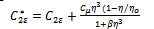
Where and , and the model constants were prescribed as:

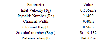
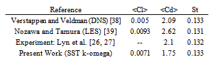
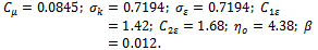The third and final turbulence closure model used in this study is the SSTKW turbulence model. It was designed by Menter [35] to give improved accuracy in terms of the onset and the amount of flow separation under adverse pressure gradients by the inclusion of the transport turbulent shear stress within the formulation of the eddy-viscosity. Additionally, the model includes a cross-diffusion term in the ω-equation and a blending function to ensure that the model equations perform reasonably within both the near-wall and far-field regions. The performance of this model, particularly with respect to shear separated flows, has been demonstrated in a large number of validation studies, including those of Bardina et al.[37].

A square cylinder of side length D (D=0.04m) was situated within a domain of size 21.5D x 14Dx 4D, as shown in Figure 1. As indicated, the square cylinder was located 4.5D aft of the inlet cross section. From previous studies[38,39], the dimensions of the computational domain were deemed sufficiently large to allow for adequate flow evolution in all directions and thus minimize boundary condition effects. A summary of some of the various geometric, inlet and non-dimensional parameters applicable to this study are shown in Table 1.

Table 1. Parameters used in the validation simulations and the experiments of Lyn et al.[26, 27]

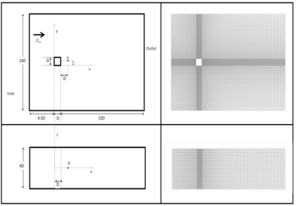Figure 1. The geometry and mesh of the square cylinder validation case Lynn et al.[26, 27]. Based on the rectangular side length D (where D=0.04m), a domain of size 21.5D x 14Dx 4D was formed. Two different, non-uniform, hexagonal mesh densities were created; the first was composed of 130x120x20 cells (y+ =100), and the second was composed of 180x180x40 cells (y+ = 30)

In order to evaluate the effect of mesh resolution, two different, non-uniform, hexagonal mesh densities were created. The first composed of 130x120x20 cells, consisted of a graded mesh near the cylinder walls conditioned on a first cell height of approximately 0.003 m. This resulted in a value for y+ of approximately 100 (well within the desired bounds for log law applications 30 < y⁺< 500). The second mesh, composed of 180x180x40 cells, was assigned a first wall cell height of 0.001 m which resulted in a viscous wall unit of approximately y⁺ = 30.

The boundary conditions consisted of a constant velocity inlet, at x = -4.5D of 0.535 m/s which resulted in a Reynolds number of 21400 (based on D). The top and bottom planes corresponding to z= ± 2D were assigned symmetry boundaries, while the lateral planes (y= ± 7D) were assigned free slip boundaries. The outlet boundary maintained a constant pressure condition corresponding to 0 Pa (Gauge) and a zero velocity gradient was imposed. The faces of square cylinder were assigned no-slip conditions.

The inlet turbulence values associated with the turbulent kinetic energy (k), the turbulent dissipation rate (ε), and the specific dissipation rate (ω) were computed from the following, approximate relations[23, 36]:

(4)

(5)

(6)

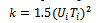
where U_i is the inlet velocity, T_i is the turbulence intensity (), and the turbulence length scale (L) was taken as 0.07d, (the factor 0.07 is based on the maximum mixing length in a turbulent pipe flow).

The governing equations were solved utilizing OpenFOAM[40] which incorporates the Finite Volume Method (FVM), in which the domain is subdivided into a finite number of small control volumes. FVM uses the integral form of a general convection-diffusion equation over a solution domain subdivided into a finite number of control volumes. For each control volume this equation may be represented as:

(7)

where ϕ is a flow variable, V is a control volume, S its bounding surface, n is a unit normal, Γ is the diffusion coefficient and q is an external force terms. The centroid of each control volume is assigned to be the computational node at which the variable values are to be calculated. Interpolation is used to express variable values at the control volume surface in terms of the centroid nodal values. Surface and volume integrals are approximated using suitable discretization methods. In this work, interpolation to cell faces for the convection terms was performed using a second-order, upwind discretization scheme, while second-order central differences were utilized for the viscous terms. Pressure-velocity coupling was based on the Pressure Implicit with Splitting of Operators (PISO) method[41]. A more detailed description of the Finite Volume Method can be found in[36].

Temporal discretization was conducted using a second order, implicit, backward differencing scheme, and a time step of 1.0e-4 seconds was selected in order to maintain the maximum Courant number below 0.5. Time averaging of the unsteady results was conducted subsequent to obtaining steady oscillatory amplitudes (typically after 10 seconds of simulation time), and was averaged over a minimum of 5 oscillation cycles.

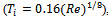
Figure 2. The time averaged, streamwise velocity component along the domain centerline (, y/D=0.5, z/D=0) comparing the SKE, RNGKE, and the SSTKW turbulence closure models with the experiments performed by Lynn et al.[26, 27](1994, 1995). The SSTKW model with near wall resolution, y+=30, resulted in the closest agreement with experiment

3. Validation Results

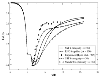
Figure 2 shows the time averaged, streamwise velocity component along the domain centerline ( y/D=0.5, z/D=0) comparing the SKE, RNGKE, and the SSTKW turbulence closure models with the experiments performed by Lynn et al.[26,27]. Unless specified otherwise, each of the models were run with the same mesh density, 130 x 120 x 20 cells, corresponding to a near wall resolution of y+=100. As indicated, there is near perfect agreement between the experimental results and all of the turbulence models forward of x/D = 0 (corresponding to the front leading edge of the square cylinder). Aft of the cylinder, (at x/D=1) however, there is noticeable disagreement. As shown, of all the models, the SKE model shows the least agreement with the experimental results. The SKE model predicts the location (x/D) and magnitude (U/Uo) of the minimum velocity to be approximately -0.1 and 2.5, respectively. This is in significant contrast to the experimental results, for which the location and the minimum velocity were measured to be approximately -0.2 and 1.25, respectively. Additionally, the rate at which the velocity returns to its free stream value is also much slower for the SKE model than for all of the other models. The RNGKE model shows some improvement both with respect to the minimum velocity magnitude (-0.18) and a steeper velocity gradient, but the location of the minimal velocity (at ~ x/D=2.5) remains unchanged from the SKE prediction. The SSTKW model with near wall resolution y+ = 100, shows better agreement with experiment than either the SKE or the RNGKE models. It predicts a minimal velocity of approximately -0.2 at a location of 1.7. The return to the free stream velocity is also faster than either model. Increasing the total number of grid elements to 180x180x40 cells, and the near wall resolution to y+=30, (corresponding to the maximum near wall resolution for which log-wall functions remain valid) resulted in better agreement with the experimental data. 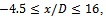As indicated, although the SSTKW at y+=30 (hereafter SSTKW2) still under predicts the streamwise velocity aft of x/D=4, the near-wall agreement () is significantly improved.

Figure 3 shows velocity and turbulent kinetic energy contours for the simulated square cylinder using SSTKW2. As shown, the vortex shedding motion is well captured. In agreement with the results of Tritico and Hotchkiss[12], who performed physical experiments on actual boulder obstructions, the initial vortex diameters are consistent with the primary obstruction dimensions.

Figure 4 shows the time history of the lift and drag coefficients, Cl and Cd, respectively, for SSTKW2. From Figure 4(a), the Cl gradually increases its amplitude of oscillation until approximately t=10s, at which time it reaches a steady oscillation amplitude of approximately ±1. Also from Figure 4(a), the oscillation period was calculated to be 0.5621 seconds, corresponding to a shedding frequency (f) of 1.779 Hz. This resulted in a Strouhal number of 1.33. Figure 4(b) shows the corresponding Cd plot over the same time interval. As indicated, the Cd plot does not show the same amplitude of oscillation as the Cl plot, but instead shows a relatively constant value through the initial 5 seconds of simulation, and thereafter a steady increase in magnitude to an approximate average value of 1.75. At this average value, the amplitude of oscillation is approximately ±0.035.

Figure 3. Contours of velocity (a) and turbulent kinetic energy (b) for the simulated square cylinder using SSTKW2 (Ui=0.535m/s; Re=2.14E4). As shown, the vortex shedding motion is well captured. Further, in agreement with the results of Tritico and Hotchkiss (2005), the initial vortex diameters are consistent with the primary obstruction dimensions

Figure 4. Time history of the lift and drag coefficients, Cl and Cd, respectively, for SSTKW2. From Figure (a), the Cl oscillation period is 0.5621 seconds, corresponding to a shedding frequency (f) of 1.779 Hz and a Strouhal number of 1.33. From Figure (b) the Cd plot shows minimal oscillations (0.035) with an average magnitude of 1.75

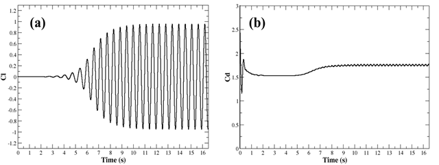
Figure 5. Geometries (lengths shown in meters) and corresponding complexity factors associated with LWD_1, LWD_2, and LWD_3. From Figure (a), LWD_1 represents the simplest (coarsest) geometric approximation of the fallen tree, while LWD_3 (Figure (c)) represents the closest (most detailed) approximation. Although LWD_1 and LWD_2 do not maintain consistent volume to surface area ratios with LWD_3, the primary dimensions of each LWD (corresponding to length, width, and height) are consistent, and constrained within the prescribed dimensional limits

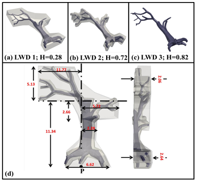
Figure 6. Merced River domain mesh and representative LWD surface mesh (corresponding to LWD_3). Figure (b) shows the cross-stream variation in turbulence kinetic energy for LWD_2 utilizing SSTKW to illustrate the sensitivity of the numerical results to grid resolution. A similar procedure was used for the remaining cases. The resulting mesh densities for LWD_1, LWD_2, and LWD_3 resulted in 2.69E5, 4.32E5, and 1.49E6 total elements, respectively, and corresponded to30≤y+≤100

Table 2 shows comparisons of the average values of Cl, Cd and St utilizing the experimental work of Lyn et al.[26, 27], as well as DNS and LES simulations conducted by Verstappen and Veldman[38], and Nozawa and Tamura[39], respectively. As shown, the Strouhal number predicted by the use of the SSTDW2 model compares favorably with both the experimental and numerical values. The Cl value was also shown to be within the range predicted by the LES and DNS numerical results. The Cd value, however, was predicted at a somewhat lower value than either the experimental or numerical comparison results. This could be attributed either as a deficiency of the model itself, or possibly the use of wall functions to approximate the pressure distribution within the turbulent boundary layer. A future study may incorporate the use of a highly resolved wall boundary, near y+=1, to ascertain the validity of this last assumption.

Table 2. Comparisons of average Cl, Cd and St between the present study and the indicated experimental/numerical work

Despite the low drag coefficient however, the overall predictive capability of the SSTW2 model was surprisingly good, particularly with respect to its predictions of stream- wise velocity, the lift coefficient, and the vortex shedding frequency (leading to the experimentally validated Strouhal number). For these reasons, the model was deemed adequate for use with the more complex LWD geometries.

4. Large Woody Debris Method

For context, we selected bathymetric field measurements taken from a 2.4-km (1.5-mile) stretch along the Robinson Restoration project of the Merced River in California[42]. This particular restoration effort was due to the decline over the last decade of both spawning and rearing of fall-run Chinook salmon[42]. A small section of this stretch was considered, extending, as shown in Figure 8(a), over an area of approximately 350 m 200 m. At approximately the 300-m, 150-m downstream location (marked A in Figure 6 (a)), one of a total of three LWD’s (Figure 5 (a-c)) was embedded within the underlying river bathymetry.

The river topography was created from a triangulated network of digital terrain mapped (DTM) data in x, y, z format. The points consisted of a coarse set of river cross-sections containing elevations and planar information in Universal Transverse Mercator (UTM) coordinates. The points were then mapped to a grid using the method outlined in a previous study[43]. In brief, the 3DS MAX[44] software tool was heavily utilized and enabled the development of a highly refined uniformly meshed surface mesh.

The boundary conditions consisted of a constant velocity inlet of 0.5 m/s. Using the approximate diameter of the tree trunk (2.28 m), this resulted in an average Reynolds number of 21400. Since the water surface elevation did not significantly change over the study section, and since this study is focused on a fully submerged bluff body, the closed lid approach was utilized to model the water surface in lieu of a free surface approach, such as the Volume of Fluid (VOF) method[45]. The outlet boundary condition was implemented using a zero velocity gradient and a constant pressure condition . The terrain boundaries, including the LWD object, were modeled with no-slip boundaries. Bed roughness was approximated from the average sediment sizes which are common to the area (~0.01m), and this roughness height was provide as an input to the turbulent viscosity via a roughness wall function approach[40]. Like the validation studies, the inlet turbulence values associated with the turbulent kinetic energy (k), the turbulent dissipation rate (ε), and the specific dissipation rate (ω) were computed from Equations 4-6.

Each LWD geometry was meshed using GAMBI [46], applying a hybrid, non-conformal combination of unstructured tetrahedral and hexahedral elements. A size function application was utilized that allowed for localized mesh refinement at the surface of each LWD. The graded mesh, governed by a first cell height of approximately 0.003 m, resulted for the case of each LWD, a value for the non-dimensional viscous wall unit (y+) of approximately 100 (well within the desired bounds for log law applications 30 < y⁺< 500). Mesh coarsening of surrounding cells was based on a 10 percent maximum successive increase and culminated in a maximum allowable edge length of approximately 0.61 m. In this manner, the face geometries having the smallest length scales governed the initial size function parameter. For each case a mesh convergence study was conducted to establish the minimum mesh resolution corresponding to grid-independent fluid dynamics. Figure 6(b) shows the cross-stream variation in turbulence kinetic energy associated with the grid resolution of LWD_2. The sampled location pertains to a distance of approximately 0.5D upstream from the obstruction. The mesh resolution, as indicated, beginning with 1.71E5 elements was first increased by a factor of approximately 2.5 to 4.32E5 elements. Subsequently a refinement factor of approximately 1.75 was employed and substantiated sufficient grid independence involving 4.32E5 elements. This same procedure was conducted for the remaining LWD cases, resulting in approximately 2.69E5 elements and 1.49E6 elements for LWD_1 and LWD_3, respectively.

From the previous validation results, the SSTKW turbulence closure method was selected due to its superior performance, over the other two turbulence models, for predicting the flow-field evolution over a rectangular cylinder. The governing equations, consisting of the conservation of mass, momentum and the two additional turbulence transport equations, were solved utilizing OpenFOAM[40]. The interpolation to cell faces for the convection terms was performed using a second-order, upwind discretization scheme, while second-order central differences were utilized for the viscous terms. Pressure-velocity coupling was based on the Pressure Implicit with Splitting of Operators (PISO) method[41]. The temporal discretization was conducted using a second order, implicit backward differencing scheme, and an average time step of 1.0e-3 seconds was adaptively maintained in order to keep the maximum Courant number below 1.0. Time averaging of the unsteady results were conducted subsequent to two flow through times (residence times), or 1.4E6 iterations.

In contrast to the validation cases, prior to conducting simulations via the highly sensitive SSTKW model, it was necessary to begin each of the three LWD simulations using the SKE approach, approximating the input values for k and epsilon from Equation 4 and Equation 5. After several seconds of simulation, an approximate value for omega could be computed based on Equation 6. In this manner, convergence and numerical instability issues were successfully avoided.

5. Geometric Complexity

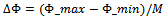
Apart from the apparent qualitative geometric differences between LWD_1, LWD_2, and LWD_3, it is desirable, for the purposes of making quantitative comparisons, to prescribe for each LWD a unique shape complexity factor. Information theory[47] is a useful tool for this purpose. The theory provides a meaningful way to quantify information and describe it within a probabilistic framework. Researchers have applied the theory, for example, to such diverse fields as communications[47], signal processing[48], and medical imaging[49].

From information theory[47] we may define a random variable x with a probability density function p(x). We define the complexity factor (H) as:

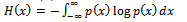(8)

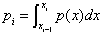Here we assume that p(x) is a continuous function, and H may be expressed in units of bits (if the log function is of base 2). If we discretize p(x) such that where x_i and x_i+1 are specific values of x we can write a discrete form of Equation (3) and obtain the following expression for the complexity factor:

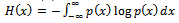(9)

In order to compute the probability density functions (p_i) in three dimensions, we may utilize Gaussian curvature, specifically the Gauss-Bonnet scheme[50,51], in which the use of the angle excess formula approximates the principal curvature of a surface

(10)

where Φ_j is the angle excess for vertex j, and the angle ϕ_i is the wedge subtended by the edges of a triangle whose corner is at the vertex of interest (Figure 5 (e)). The angle excess for each vertex (valid for two or three dimensions) can then be distributed among M bins with bin width:

(11)

and probability density:

(12)

where is the number of Φ_j samples that fall within Φ_min + (i – 1) ΔΦ ≤ Φ_j < Φ_min + iΔΦ, and N is the total number of samples over the surface.

To illustrate this process, consider the two dimensional segmented square shown in Figure 5 (b). As shown, the figure is made up of a total of 24 sample points with four samples at the corners and 20 sample points along the flat edges. The total number of bins (B_i) is thus two and are composed of the corner samples, each having an angle (based on the two adjacent line segments) of 90 degrees, and the flat segments with angles corresponding to 180 degrees. Thus the probability density (Equation 12) for each of the two bins is: , and, respectively. Applying Equation 4 (and ensuring log₂x is utilized), this leads to a complexity factor of 0.65 bits. By comparison, the decagon of Figure 7(a) contains only one bin for all of its N=10 samples. This figure thus yields a complexity factor of zero, and provides an idealized reference value from which all other shapes (with equivalent samples; N=10) may be compared. Figure 5 (c-d) shows the complexity factors associated with two additional shapes with increasing levels of complexity. As shown, even though the total number of samples remains the same (a necessary prerequisite for making relative comparisons among 2D and 3D objects), the asymmetry of Figure 7(d) contributes to its having a higher complexity factor.

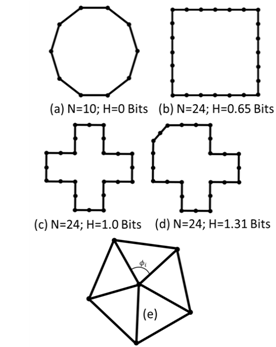Figure 7. Two dimensional segmented objects used to illustrate the method of computing the complexity factor. Each object of sample size (N) is shown in order of increasing complexity. As shown in (c) and (d), even though the number of total number of samples remains the same, the asymmetry of (d) contributes to one additional bin (), and thus an overall increase in complexity factor. Figure (e) illustrates the angle , associated with a three dimensional wedge subtended by the edges of a triangle whose corner is at a vertex. This is used to approximate the three Dimensional surface curvature via the excess angle formula

For three dimensional surfaces, the process is nearly equivalent to that of two dimensions. The only exception is that the number of bins are computed using Equation 5 in order to compute the angle excess. Additionally, as a point of reference, the analog to the 2D uniform polygon, with null complexity factor, is a regular sphere.

Since the bin width () and sample size (N) govern the computation of the probability density function (and thus the complexity factor), for relative comparisons among each LWD, we must use consistent numbers of each. For this work we used a constant bin width of 1 deg (M = 360°) and a sample size (N), corresponding to the total number of boundary vertices of LWD_1 (N=24,825).

6. Length Scale

The global Reynolds number (Re) is commonly defined as:

(13)

where U_∞ is the free-flow velocity, L represents a global length scale, and ν (m²/s) is the kinematic viscosity. The choice of length scale, except for the most idealized geometries, is somewhat arbitrary. Complex geometries (i.e., the LWD’s presented here) often render the selection of a global length scale entirely arbitrary. Since this study is focused on the localized effect of the LWD on the flow field, and provides a quantitative estimate of the shape complexity, a more accurate representation of the length scale is warranted.

We may define a local length scale (L_i), evaluated at each LWD surface cell[52] as:

(14)

where Q is representative of any scalar flow field quantity. In this work we have chosen to utilize the turbulent kinetic energy (k) in conjunction with the localized cell velocity (U_i). The local Re is thus:

(15)

7. Large Woody Debris Results

The resulting complexity factors for each LWD are shown in Table 3. As expected, LWD_1 exhibits the least shape complexity with a complexity factor value of 0.28 bits, while LWD_2 and LWD_3 have complexity factor values of 0.72 bits and 0.82 bits, respectively. The probability plot shown in Figure 8 helps to further clarify the complexity factor differences. As indicated from Figure 8(a), a significant proportion of the LWD bin probabilities are associated with bin 1, corresponding to planar surfaces. Bin one, for example accounts for nearly 85% of LWD_1 surfaces and approximately 72% and 50% for LWD_2 and LWD_3, respectively. Since the remainder of the vertex angles (bins) are associated with non-planar surfaces, it is evident from Figure 8(b), that LWD_2 and LWD_3 contain a much larger proportion of these bin probabilities compared to LWD_1. This larger variance directly corresponds to the increase in complexity factor for LWD_2 and LWD_3. Additional studies of the three LWD’s incorporating larger sample sizes and more refined bin widths were conducted and resulted in negligible complexity factor changes.

Table 3. Complexity factor (bits) and surface area for each simulated LWD

Figure 9 shows the velocity and turbulent kinetic energy (TKE) contours for each LWD along the z-axis midplane. As shown, qualitative differences for each LWD on the surrounding flow field are readily identifiable. While LWD_1 and LWD_2 maintain relatively high-velocities and TKE’s along their left and right peripheral edges, LWD_3 by comparison shows a significantly more uniform distribution of velocity and TKE. Further, while each LWD shows signs of a wake effect (characterized by a sudden decrease in velocity) aft of the root bulb and at each submerged branch location within the z-axis plane shown, there is a significant difference in the relative size of each wake and its corresponding velocity and/or TKE magnitude. The results clearly indicate that LWD_3 appears to be far less obstructive to the flow field than either LWD_1 or LWD_2.

Figure 8. Plots showing LWD _1, LWD_2, and LWD_3 bin probabilities used for calculating the shape complexity factor. While a significant proportion of the LWD bin probabilities are associated with bin 1 (see Figure (a)), which corresponds to planar surfaces, LWD_2 and LWD_3 contain a relatively larger proportion of bin probabilities associated with additional vertex angles. These angles correspond to various curved surfaces (see Figure (b)). This variance directly corresponds to the increase in complexity factor for LWD_2 and LWD_3

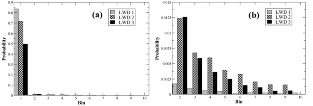
Figure 9. Velocity and TKE contours for each LWD about the z-axis midplane. As shown in Figures (a) through (d), the simplistic representations (LWD_1, and LWD_2) result in high velocity, high TKE, peripheral flow fields which surround relatively large wake regions. By comparison, LWD_3 shows significantly smaller wake regions and increased overall uniformity of velocity and TKE

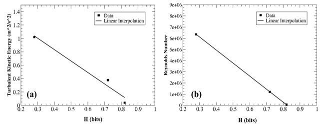Figure 10. Plots of locally integrated TKE and Reynolds number (Re) as a function of complexity factor (H). As shown, both the TKE and Re decrease linearly with increasing object complexity

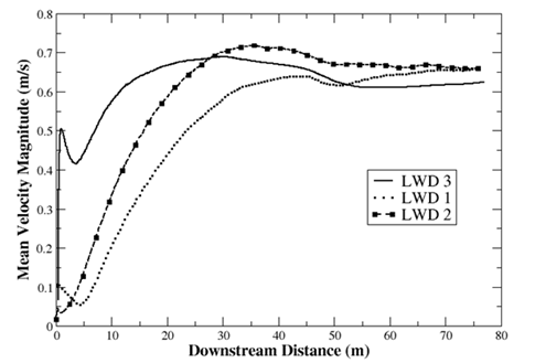Figure 11. Time averaged velocity magnitude for each LWD extending aft of the root wad approximately 30D downstream (z-axis midplane). LWD_1 shows the lowest velocity magnitude forward of 12D corresponding to the larger wake influence, while LWD_3 shows the highest velocity magnitude, corresponding to smaller wake influence. The velocities for each LWD begin to converge aft of approximately 16D

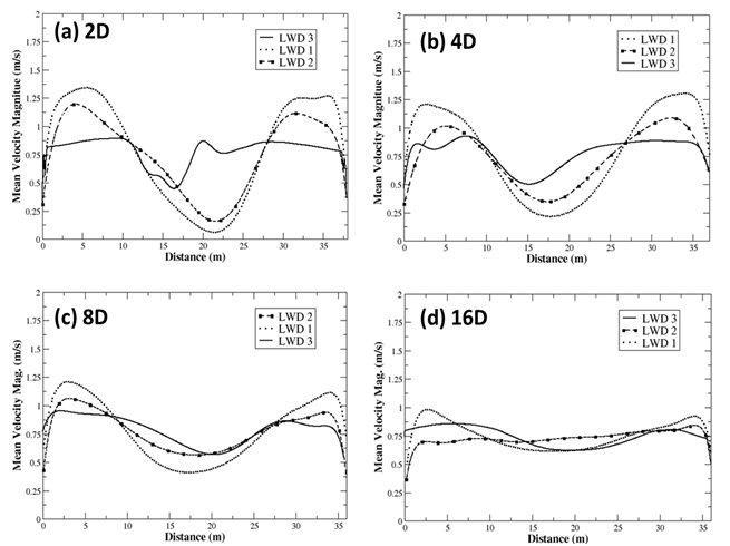Figure 12. Time averaged velocity magnitude for each LWD corresponding to four downstream, cross-section locations; 2D, 4D, 8D and 16D (z-axis midplane). As shown in Figure (a) at a downstream distance of 2D, LWD_3 shows a significant variation in the flowfield within the wake region, directly aft of the complex root bulb. Flowfield variation (particularly evidence of the root bulb wake) begins to significantly diminish at 16D

Figure 10 shows the relationship between the locally integrated values for TKE and Re as functions of complexity factor (H). The integration was performed over each LWD surface, and in the case of the Re, was performed in accordance with Equation 15. Tabulated values for these integrations are shown in Table 3. From Figure 10(a), for the three LWD cases studied, the TKE decreases linearly with an increase in the complexity factor. This result is not surprising due to the increased pressure drag that generally dominates any skin friction drag for high Re flows over bluff bodies. The fact that LWD_1’s surface area is approximately 216% larger than that of LWD_3 accounts for the increased pressure drag of LWD_1. Further, since increases in TKE are in general, associated with increases in Re, this same trend is also present in Figure 10(b).

Figure 11 compares the time averaged velocity magnitude (U_mag) for each LWD along a downstream location beginning aft of the root bulb (see point P of Figure 7) and extending approximately 30D (75 m) to the end of the computational domain. As indicated, LWD_1 shows the lowest velocity magnitude forward of 12D corresponding to its larger wake influence behind the root bulb, while LWD_3 shows the highest velocity magnitude. The velocities for each LWD begin to converge aft of approximately 16D. Another distinguishing feature corresponds to the LWD velocity within the first couple of meters of downstream distance. As shown, LWD_3 shows a dramatic velocity increase of 0.5 m/s, while LWD_1 and LWD_2 show either no increase, or in the case of LWD_1, a small decrease in velocity within this initial distance. This disparity can be attributed to the fact that the root bulb geometry corresponding to LWD_3 was not modeled as a blunt, termination (as was partly the case for LWD_2, and completely the case for LWD_1), but rather a more realistic agglomeration of root extensions (see Figure 7). This would allow for less flow reversal, and the higher, overall velocity magnitudes shown.

Figure 12 compares the time averaged velocity magnitude (U_mag) for each LWD at four different downstream locations (2D, 4D, 8, 16D) located aft of the root bulb (see point P of Figure 7). The plots are shown with cross-stream distances measured from the right bank to the left bank (facing downstream). First observations reveal that the wake effect, illustrated by the sudden decrease in velocity directly aft of the LWD, diminishes with downstream distance. This can be quantified by measuring the velocity difference (δ_v) between the global maxima and global minima (excluding the endpoints). For LWD_1, the range ofδ_v decreased from 1.3 m/s to 0.38 m/s, between downstream distances of 2D and 16D, respectively. LWD_2 shows a decrease from 1.13 m/s to 0.19 m/s and LWD_3 shows a decrease from 0.49 m/s to 0.25 m/s. The respective magnitudes of these results substantiate a second general observation, revealing unsurprisingly (due to its larger surface area), that, outside the wake region, LWD_1 maintains the highest overall peak velocities, while LWD_1 maintains the lowest overall peak velocities. Inside the wake region (between 10m and 27.5 m), with the exception of the downstream distance of 16D, the conditions are reversed, with LWD_1 showing the lowest overall velocities, and LWD_3 maintaining the highest overall velocities. Concerning more localized observations, Figure 12 (a), corresponding to a downstream distance of 2D, clearly reveals the influence of modeling simplification on the flow-field. As indicated, LWD_3 shows a sudden decrease in velocity at approximately 10 m which plateaus at 0.625 m/s to approximately 15 m. This velocity again dips to 0.5 m/s before again climbing to 0.875 m/s at 20 m. Thereafter over a distance of approximately 7.5 m another small change in velocity occurs before it finally begins to stabilize at approximately 27.5 m. As shown in Figure 12 (a), apart from a minor change in slope between 10m and 15m by LWD_2, this velocity variation, is clearly not evident in either LWD_2 or LWD_3. Signs of this velocity variation continue for LWD_3 at the 4D downstream distance (Figure 12(b)). Although significantly diffused, this flow-field variation within the wake region provides an important indication of the effect that modeling details have on the downstream flow-field.

8. Summary and Conclusions

The purpose of this article was to evaluate the effect of LWD geometric simplification on the flow-field dynamics as evaluated using CFD. The first step included a validation effort with existing experimental data on two relatively simple boulder geometries consisting of an idealized cylindroid and parallelepiped. The validation tests resulted in reasonable agreement between the numerical and experimental results for both the streamwise velocity and turbulent kinetic energy at a given 1-m cross section. Next a series of three LWD case studies were examined, each representing the same LWD object, but consisting of progressively finer geometric resolution. For each LWD a shape complexity factor was computed based on Information Theory and used quantitatively for relative complexity comparisons. As expected, the localized effect of increased Re resulted in an increase in turbulent kinetic energy. However, for the cases examined, an increase in complexity factor resulted in local decreases in turbulent kinetic energy. The effect of geometric complexity on the velocity magnitude and turbulent kinetic energy was also evident on the downstream flow field. The results indicated that minimizing complexity can result in significant over predictions of both velocity magnitude and turbulent kinetic energy.

In summary, the localized and downstream effects of oversimplifying LWD objects within a computational flow field simulation can be significant. Caution should be exercised when undertaking prediction efforts to quantify the effects of these structures when any degree of geometric simplification is conducted.

ACKNOWLEDGEMENTS

This study was funded in part through the System-wide Water Resources Program (SWWRP).

Nomenclature

B_i Sampling parameter

C_μEmpirical constant used in k-ε model

d Semi-major axis (m)

H Complexity factor (bits)

k Turbulent kinetic energy (m²/s²)

k_s Roughness length (m)

L Length scale (m)

LWD Large woody debris

M Number of bins

N Total number of samples

p_iProbability density

Q Representative scalar flow quantity

Re Reynolds number

T_iTurbulence intensity

UVelocity (m/s)

Greek Symbols

Bin width

Angle excess (deg.)

ε Turbulent dissipation rate (m²/s³)

ϕ Subtended wedge angle (deg.)

v Kinematic viscosity (m²/s)

Subscripts

mag magnitude

∞ freestream