1. Introduction

In the process of developing the technology, many possible interesting adaptations became apparent: One of the most interesting directions was the use of the technology in the analysis of long DNA sequences. A benefit of the techniques was that it combined rigorous statistical analysis with modern computer power to quickly search for diagnostic patterns within long DNA sequences. Briefly, a DNA strand can be viewed as a long string of linked nucleotides. Each nucleotide is composed of a nitrogenous base, a five carbon sugar, and a phosphate group. There are four different bases that can be grouped by size, the pyrimidines, thymine (T) and cytosine (C), and the purines, adenine (A) and guanine (G). The nucleotides are linked together by a backbone of alternating sugar and phosphate groups with the carbon of one sugar linked to the carbon of the next, giving the string direction. DNA molecules occur naturally as a double helix composed of polynucleotide strands with the bases facing inward. The two strands are complementary, so it is sufficient to represent a DNA molecule by a sequence of bases on a single strand; refer to Fig. 1. Thus, a strand of DNA can be represented as a sequence 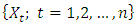of letters, termed base pairs (bp), from the finite alphabet The order of the nucleotides contains the genetic information specific to the organism. Expression of information stored in these molecules is a complex multistage process. One important task is to translate the information stored in the protein-coding sequences (CDS) of the DNA[Stoffer (2012].

Figure 1. The general structure of DNA and its bases

A common problem in analyzing long DNA sequence data is in identifying CDS that are dispersed throughout the sequence and separated by regions of noncoding (which makes up most of the DNA). Another problem of interest that we will address here is that of matching two DNA sequences, say and . The background behind the problem is discussed in detail in the study by Waterman and Vingron (1994). For example, every new DNA or protein sequence is compared with one or more sequence databases to find similar or homologous sequences that have already been studied, and there are numerous examples of important discoveries resulting from these database searches.

One naive approach for exploring the nature of a DNA sequence is to assign numerical values (or scales) to the nucleotides and then proceed with standard time series methods. It is clear, however, that the analysis will depend on the particular assignment of numerical values. Consider the artificial sequence ACGTACGTACGT. . . Then, setting A = G = 0 and C = T = 1, yields the numerical sequence 010101010101. . . , or one cycle every two base pairs (i.e., a frequency of oscillation of Cycle/bp, or a period of oscillation of length bp=cycle). Another interesting scaling is A = 1, C = 2, G = 3, and T = 4, which results in the sequence 123412341234. . . , or one cycle every four bp In this example, both scalings of the nucleotides are interesting and bring out different properties of the sequence. It is clear, then, that one does not want to focus on only one scaling. Instead, the focus should be on finding all possible scalings that bring our interesting features of the data. Rather than choose values arbitrarily, the spectral envelope approach selects scales that help emphasize any periodic feature that exists in a DNA sequence of virtually any length in a quick and automated fashion. In addition, the technique can determine whether a sequence is merely a random assignment of letters [Stoffer (2012)].

Fourier analysis has been applied successfully in DNA analysis; McLachlan and Stewart (1976) and Eisenberg et al. (1994) studied the periodicity in proteins using Fourier analysis.

Stoffer et al. (1993) proposed the spectral envelope as a general technique for analyzing categorical-valued time series in the frequency domain. The basic technique is similar to the methods established by Tavar´e and Giddings (1989) and Viari et al. (1990), however, there are some differences. The main difference is that the spectral envelope methodology is developed in a statistical setting to allow the investigator to distinguish between significant results and those results that can be attributed to chance.

The article authored by Marhon and Kremer 2011, partitions the identification of protein-coding regions into four discrete steps. Based on this partitioning, digital signal processing DSP techniques can be easily described and compared based on their unique implementations of the processing steps. They compared the approaches, and discussed strengths and weaknesses of each in the context of different applications. Their work provides an accessible introduction and comparative review of DSP methods for the identification of protein-coding regions. Additionally, by breaking down the approaches into four steps, they suggested new combinations that may be worthy of future studies. A new methodology for the analysis of DNA/RNA and protein sequences is presented by Bajic in 2000. It is based on a combined application of spectral analysis and artificial neural networks for extraction of common spectral characterization of a group of sequences that have the same or similar biological functions. The method does not rely on homology comparison and provides a novel insight into the inherent structural features of a functional group of biological sequences. The nature of the method allows possible applications to a number of relevant problems such as recognition of membership of a particular sequence to a specific functional group or localization of an unknown sequence of a specific functional group within a longer sequence. The results are of general nature and represent an attempt to introduce a new methodology to the field of biocomputing. Fourier transform infrared (FTIR) spectroscopy has been considered by Han et al. in 2018 as a powerful tool for analysing the characteristics of DNA sequence. This work investigated the key factors in FTIR spectroscopic analysis of DNA and explored the influence of FTIR acquisition parameters, including FTIR sampling techniques, pretreatment temperature, and sample concentration, on calf thymus DNA. The results showed that the FTIR sampling techniques had a significant influence on the spectral characteristics, spectral quality, and sampling efficiency. A novel clustering method is proposed by Hoang et al. in 2015 to classify genes and genomes. For a given DNA sequence, a binary indicator sequence of each nucleotide is constructed, and Discrete Fourier Transform is applied on these four sequences to attain respective power spectra. Mathematical moments are built from these spectra, and multidimensional vectors of real numbers are constructed from these moments. Cluster analysis is then performed in order to determine the evolutionary relationship between DNA sequences. The novelty of this method is that sequences with different lengths can be compared easily via the use of power spectra and moments. Experimental results on various datasets show that the proposed method provides an efficient tool to classify genes and genomes. It not only gives comparable results but also is remarkably faster than other multiple sequence alignment and alignment-free methods. One challenge of GSP is how to minimize the error of detection of the protein coding region in a specified DNA sequence with a minimum processing time. Since the type of numerical representation of a DNA sequence extremely affects the prediction accuracy and precision, by this study Mabrouk in 2017 aimed to compare different DNA numerical representations by measuring the sensitivity, specificity, correlation coefficient (CC) and the processing time for the protein coding region detection. The proposed technique based on digital filters was used to read-out the period 3 components and to eliminate the unwanted noise from DNA sequence. This method applied to 20 human genes demonstrated that the maximum accuracy and minimum processing time are for the 2-bit binary representation method comparing to the other used representation methods. Results suggest that using 2-bit binary representation method significantly enhanced the accuracy of detection and efficiency of the prediction of coding regions using digital filters. Identification and analysis of hidden features of coding and non-coding regions of DNA sequence is a challenging problem in the area of genomics. The objective of the paper authored by Roy and Barman in 2011 is to estimate and compare spectral content of coding and non-coding segments of DNA sequence both by Parametric and Nonparametric methods. Consequently, an attempt has been made so that some hidden internal properties of the DNA sequence can be brought into light in order to identify coding regions from non-coding ones. In this approach the DNA sequence from various Homo Sapien genes have been identified for sample test and assigned numerical values based on weak-strong hydrogen bonding (WSHB) before application of digital signal analysis techniques. The statistical methodology applied for computation of Spectral content are simple and the Spectrum plots obtained show satisfactory results. Spectral analysis can be applied to study base-base correlation in DNA sequences. A key role is played by the mapping between nucleotides and real/complex numbers. In 2006, Galleani and Garello presented a new approach where the mapping is not kept fixed: it is allowed to vary aiming to minimize the spectrum entropy, thus detecting the main hidden periodicities. The new technique is first introduced and discussed through a number of case studies, then extended to encompass time-frequency analysis.

For analyzing periodicities in categorical valued time series, the concept of the spectral envelope was introduced by Stoffer et al., 1993 as a computationally simple and general statistical methodology for the harmonic analysis and scaling of non-numeric sequences. However, The spectral envelope methodology is computationally fast and simple because it is based on the fast Fourier transform and is nonparametric (i.e., it is model independent). This makes the methodology ideal for the analysis of long DNA sequences. Fourier analysis has been used in the analysis of correlated data (time series) since the turn of the century. Of fundamental interest in the use of Fourier techniques is the discovery of hidden periodicities or regularities in the data. Although Fourier analysis and related signal processing are well established in the physical sciences and engineering, they have only recently been applied in molecular biology. Since a DNA sequence can be regarded as a categorical-valued time series it is of interest to discover ways in which time series methodologies based on Fourier (or spectral) analysis can be applied to discover patterns in a long DNA sequence or similar patterns in two long sequences. Actually, the spectral envelope is an extension of spectral analysis when the data are categorical valued such as DNA sequences.

An algorithm for estimating the spectral envelope and the optimal scalings given a particular DNA sequence with alphabet is as follows [Stoffer (2012].

1. Given a DNA sequence of length from the vectors namely, for if where is a vector with a 1 in the jth position as zeros elsewhere, and if

2. Calculate the Fast Fourier Transform FFT of the data,

Note that is a complex-valued vector. Calculate the periodogram, for and retain only the real part, say

3. Smooth the real part of the periodogram as preferred to obtain a consistent estimator of the real part of the spectral matrix.

4. Calculate the variance–covariance matrix of the data, 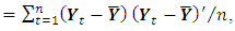where is the sample mean of the data.

5. For each determine the largest eigenvalue and the corresponding eigenvector of the matrix

6. The sample spectral envelope is the eigenvalue obtained in the previous step.

7. The optimal sample scaling is , where is the eigenvector obtained in the previous step.

In this paper, we discussed the cluster analysis of the first, second, third and fourth variance- covariance matrix eigenvalues of Fast Fourier Transform (FFT) for numerical values representation of DNA sequences of five organisms, Human, E. coli, Rat, Wheat and Grasshopper. The analysis is based on Ward’s method of clustering. It should be noted that it is the first time that the variance covariance matrix eigenvalues of Fast Fourier Transform (FFT) for numerical values representation of DNA sequences, is used in an analysis like this and related analyzes.

2. Ward’s Method of Clustering

Data clustering is a method of creating groups of objects, or clusters, in such a way that objects in one cluster are very similar and objects in different clusters are quite distinct. Data clustering is often confused with classification, in which objects are assigned to predefined classes. In data clustering, the classes are also to be defined.

Cluster analysis is widely used in biological analyzes, including DNA analysis. Some of the relevant scientific literatures are as follows.

Jiang et al. in 2004 divided cluster analysis for gene expression data into three categories. Then, they presented specific challenges pertinent to each clustering category and introduce several representative approaches. They also discuss the problem of cluster validation in three aspects and review various methods to assess the quality and reliability of clustering results.

Polovinkin et al. in 2016 deal with the problem of diagnosis of oncological diseases based on the analysis of DNA methylation data using algorithms of cluster analysis and supervised learning. The groups of genes are identified, methylation patterns of which significantly change when cancer appears. High accuracy is achieved in classification of patients impacted by different cancer types and in identification if the cell taken from a certain tissue is aberrant or normal. With method of cluster analysis two cancer types are highlighted for which the hypothesis was confirmed stating that among the people affected by certain cancer types there are groups with principally different methylation pattern.

James et al. in 2018 adapted the mean shift algorithm, an unsupervised machine-learning algorithm, which has been used successfully thousands of times in fields such as image processing and computer vision. They described the first application of the mean shift algorithm to clustering DNA sequences. They also applied supervised machine learning to predict the identity score produced by global alignment using alignment-free methods. They demonstrate MeShClust's ability to cluster DNA sequences with high accuracy even when the sequence similarity parameter provided by the user is not very accurate.

Wu et al. in 2003 described a genetic K-means clustering algorithm, called GKMCA, for clustering in gene expression datasets. The superiority of the GKMCA over other clustering algorithms is demonstrated for two real gene expression datasets.

In many biological applications it is necessary to cluster DNA sequences into groups that represent underlying organismal units, such as named species or genera. In metagenomics this grouping needs typically to be achieved on the basis of relatively short sequences which contain different types of errors, making the use of a statistical modeling approach desirable. Jaaskinen et al. in 2014 introduced a novel method for this purpose by developing a stochastic partition model that clusters Markov chains of a given order. The model is based on a Dirichlet process prior and they use conjugate priors for the Markov chain parameters which enables an analytical expression for comparing the marginal likelihoods of any two partitions. To find a good candidate for the posterior mode in the partition space, they use a hybrid computational approach which combines the EM-algorithm with a greedy search.

Guntur in 2007 in his thesis of compared among few Clustering algorithms such as: K means, Hierarchical, Self Organization Map(SOM), and Cluster A±nity Search Technique(CAST) with proposed algorithm called CAST+ for Gene Expression data. Results show that Proposed Algorithm is efficient in comparison with other Clustering algorithms mentioned above. The Clustering algorithms are compared on the basis of few Evaluation Indices such as Homogeneity Vs separation, and Silhouette width.

Liu et al. in 2018 applied comprehensive analyses of RNA-seq and CAGE-seq (cap analysis of gene expression and sequencing) to characterize the dynamic changes in lncRNA expression in rhesus macaque (Macaca mulatta) brain in four representative age groups. They identified 18 anatomically diverse lncRNA modules and 14 mRNA modules representing spatial, age, and sex specificities. Spatiotemporal- and sex-biased changes in lncRNA expression were generally higher than those observed in mRNA expression. A negative correlation between lncRNA and mRNA expression in cerebral cortex was observed and functionally validated. Their findings offer a fresh insight into spatial-, age-, and sex-biased changes in lncRNA expression in macaque brain and suggest that the changes represent a previously unappreciated regulatory system that potentially contributes to brain development and aging.

Ruiz et al. in 2018 proposed a novel approach for performing cluster analysis of DNA sequences that is based on the use of GSP methods and the K-means algorithm. They also proposed a visualization method that facilitates the easy inspection and analysis of the results and possible hidden behaviors. Their results support the feasibility of employing the proposed method to find and easily visualize interesting features of sets of DNA data.

Hard clustering algorithms are subdivided into hierarchical algorithms and partitional algorithms.

A partitional algorithm divides a data set into a single partition, whereas a hierarchical algorithm divides a data set into a sequence of nested partitions. Hierarchical algorithms are subdivided into agglomerative hierarchical algorithms and divisive hierarchical algorithms. Agglomerative hierarchical clustering starts with every single object in a single cluster. Then it repeats merging the closest pair of clusters according to some similarity criteria until all of the data are in one cluster.

The choice of distances is important for applications. The squared Euclidean distance is probably the most common distance we have ever used for numerical data. For two data points and in d-dimensional space, the squared Euclidean distance between them is defined to be,

According to different distance measures between groups, agglomerative hierarchical methods can be subdivided into graph methods and geometric methods. Ward’s method is one of geometric methods. The Ward’s method is one of the most popular method.

Ward (1963) and Ward and Hook (1963) proposed a hierarchical clustering procedure seeking to form the partitions in a manner that minimizes the loss of information associated with each merging. Usually, the information loss is quantified in terms of an error sum of squares (ESS) criterion, so Ward’s method is often referred to as the “minimum variance” method.

Given a group of data points C, the ESS associated with C is given by,

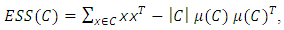Where,

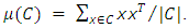Suppose there are k groups in one level of the clustering, then the information loss is represented by the sum of ESSs given by, 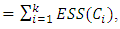which is the total within-group ESS.

At each step of Ward’s method, the union of every possible pair of groups is considered and two groups whose fusion results in the minimum increase in loss of information are merged. If the squared Euclidean distance is used to compute the dissimilarity matrix, then the dissimilarity matrix can be updated by the Lance-Williams formula during the process of clustering as follows (Wishart, 1969):

Where,

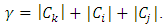To justify this, we suppose and are chosen to be merged and the resulting cluster is denoted by Then the increase in ESS is,

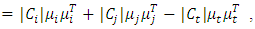Where, and are the means of clusters and respectively.

After simple mathematical operations, we get[ ],

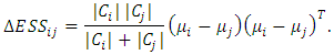Now, considering the increase in that would result from the potential fusion of groups and from the above equation, we have,

If we compute the dissimilarity matrix for a data set using the squared Euclidean distance, then the entry of the dissimilarity matrix is,

Where d is the dimensionality of the data set D.

If and then the increase in ESS that results from the fusion of and is,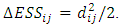

Since the objective of Ward’s method is to find at each stage those two groups whose fusion gives the minimum increase in the total within-group ESS, the two points with minimum squared Euclidean distance will be merged at the first stage. Suppose and have minimum squared Euclidean distance. Then and will be merged. After and are merged, the distances between and other points must be updated.

Now, let be any other group. If we update the dissimilarity matrix during the process of clustering, then the two groups with minimum distance will be merged. Then the increase in ESS that would result from the potential fusion of and can be calculated as,

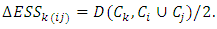A hierarchical clustering can be represented by either a picture or a list of abstract symbols. A picture of a hierarchical clustering is much easier for humans to interpret. A list of abstract symbols of a hierarchical clustering may be used internally to improve the performance of the algorithm. Some common representations of hierarchical clusterings are summarized below,

1. Dendogram: The best way to view the output of a cluster analysis is usually by looking at the Dendogram Working from the bottom up, the dendogram shows the sequence of joins that were made between clusters. Lines are drawn connecting the clustered that are joined at each step, while the vertical axis displays the distance between the clusters when they were joined. In the other words a Dendogram or valued tree is used to visualize the results of a hierarchical clustering algorithm (Gordon 1996). A dendrogram is an n-tree in which each internal node is associated with a height satisfying the condition 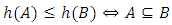for all subsets of data points

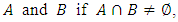Where, and denote the heights of and respectively. The heights in the dendrogram satisfy the following ultrametric conditions (Johnson, 1967),

In fact, the above ultrametric condition (7.1) is also a necessary and sufficient condition for a dendrogram (Gordon, 1987). Mathematically, a dendrogram can be represented by a function 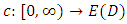that satisfies (Sibson, 1973),

is eventually in

for some small where D is a given data set and E(D) is the set of equivalence relations on D.

2. Icicle Plot: The Icicle Plot displays a schematic diagram showing members of the clusters at each stage of the algorithm. It is most useful when the number of items is small; Under each Number of Clusters is a row of X’s. Any items connected by contiguous X’s are contained in the same cluster.

An icicle plot, proposed by Kruskal and Landwehr (1983), is another method for presenting a hierarchical clustering. It can be constructed from a dendrogram. The major advantage of an icicle plot is that it is easy to read off which objects are in a cluster during a live process of data analysis.

In an icicle plot, the height and the hierarchical level are represented along the vertical axis; each object is assigned a vertical line and labeled by a code that is repeated with separators (such as “&”) along the line from top to bottom until truncated at the level where it first joins a cluster, and objects in the same cluster are joined by the symbol “=” between two objects.

3. Agglomeration Schedule: The Agglomeration Schedule provides a summary of each step in an agglomerative clustering algorithm. It is shows the amount of error created at each clustering stage when two different objects – cases in the first instance and then clusters of cases – are brought together to create a new cluster. A large jump in the value of the error term indicates that two different things have been brought together and that there is a significant typology at that level of fusion.

3. An Empirical Study

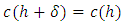
The following algorithm steps is performed to achieve our aim,

1. Generate the DNA sequence for five organisms, Human, E. coli, Rat, Wheat and Grasshopper with corresponding information in table (1).

Table (1). Relative proportions (%) of Bases in DNA

2. The sequence size is n=500 and run size is k=203.

3. Transform DNA sequence to numerical values by setting one to the base that appears and zero to the other bases.

4. Transform the sequence of numerical values to the corresponding FFT values.

5. Calculate the eigenvalues for each run results, and then we get 205 fourth order vectors of eigenvalues for each organism. Each vector contains the four eigenvalues, rank from the largest one to the smallest.

Ward’s method of clustering has been applied of the first, second, third and fourth variance- covariance matrix eigenvalues of Fast Fourier Transform (FFT) for numerical values representation of DNA sequences of five organisms, Human, E. coli, Rat, Wheat and Grasshopper. The analysis is based on Ward’s method of clustering. It should be noted that it is the first time that the variance covariance matrix eigenvalues of Fast Fourier Transform (FFT) for numerical values representation of DNA sequences, is used in an analysis like this and related analyzes.

For convenient, in the following discussions, we will refer to the organism by the first letter of his name. The number following the letter will be indicating to the order of eigenvalue (first, second, third or fourth).

3.1. For the First Eigenvalue

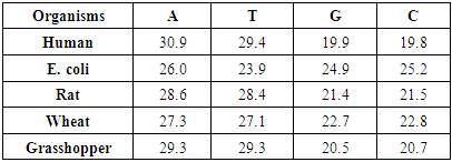
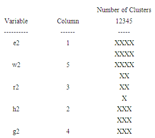
Ward’s method of clustering has created one cluster from the 203 points supplied. The clusters are groups of variables with similar characteristics. To form the clusters, the procedure began with each variable in a separate group. It then combined the two variables which were closest together to form a new group. After recomputing the distance between the groups, the two groups then closest together were combined. This process was repeated until only one group remained. The following Icicle Plot shows how the one cluster were formed. Each column of the plot shows how the variables were divided into a specific number of clusters. In that column, an unbroken string of X's connects all members of a cluster. A row without an X indicates a break between two clusters. Working from the right of this table, you can determine how the variables were combined.

The icicle plot in fig.2, shows how the one cluster were formed. Each column of the plot shows how the variables were divided into a specific number of clusters. In that column, an unbroken string of X's connects all members of a cluster. A row without an X indicates a break between two clusters. Working from the right of this table, you can determine how the variables were combined.

Figure 2. The icicle plot according to the first eigenvalue of each of five organisms

The agglomeration schedule in table (2), shows which variables were combined at each stage of the clustering process. For example, in the first stage, variable 1 was combined with variable 5. The distance between the groups when combined was 10457.8. It also shows that the next stage at which this combined group was further combined with another cluster was stage 4.

Table (2). Agglomeration Schedule for the first eigenvalue of each of five organisms

The dendrogram in fig.3, shows the hierarchical clustering structure of five organisms, Human, E. coli, Rat, Wheat and Grasshopper based on the first eigenvalue of variance- covariance matrix of Fast Fourier Transform (FFT) for numerical values representation of DNA sequences.

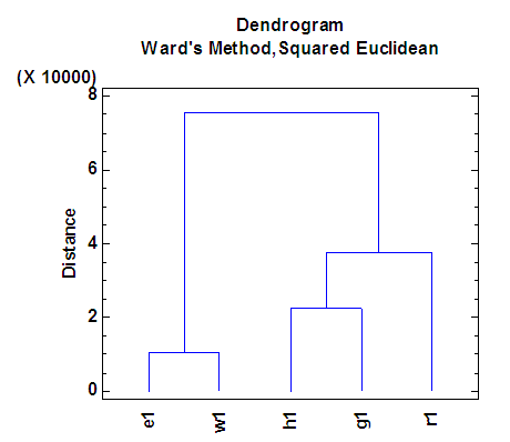Figure 3. Dendrogram according to the first eigenvalue of each of five organisms

As a result, cluster analysis based on the first eigenvalue shows that the first connection is between E. coli and Wheat. The second connection is between Human and Grasshopper. The third connection is between Human and Grasshopper from the first hand and Rat on the other. The fourth connection is between Human, Grasshopper and Rat from the first hand and E. coli and Wheat on the other.

3.2. For the Second Eigenvalue

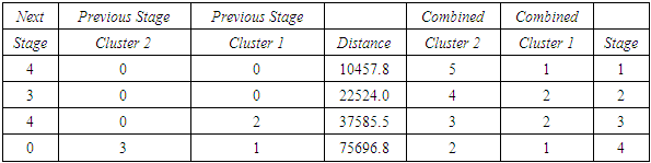
The agglomeration schedule in table (3), shows which variables were combined at each stage of the clustering process. For example, in the first stage, variable 1 was combined with variable 5. The distance between the groups when combined was 5622.44. It also shows that the next stage at which this combined group was further combined with another cluster was stage 3.

Table (3). Agglomeration Schedule for the second eigenvalue of each of five organisms

As a result, cluster analysis based on the second eigenvalue shows that the first connection is between E. coli and Wheat. The second connection is between Human and Grasshopper. The third connection is between E. coli and Wheat from the first hand and Rat on the other. The fourth connection is between E. coli, Wheat and Rat from the first hand and Human and Grasshopper on the other. Table (3) and figures 4 and 5 explain what we stated above.

Figure 4. The icicle plot according to the second eigenvalue of each of five organisms

Figure 5. Dendrogram according to the second eigenvalue of each of five organisms

It is clear that the clustering process based on the second eigenvalue differ slightly, from the connection aspect, compared with clustering process based on the first eigenvalue.

3.3. For the Third Eigenvalue

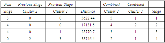
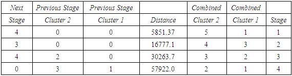
The agglomeration schedule in table (4), shows which variables were combined at each stage of the clustering process. For example, in the first stage, variable 1 was combined with variable 5. The distance between the groups when combined was 5851.37. It also shows that the next stage at which this combined group was further combined with another cluster was stage 4.

Table (4). Agglomeration Schedule for the third eigenvalue of each of five organisms

As a result, cluster analysis based on the third eigenvalue shows that the first connection is between E. coli and Wheat. The second connection is between Rat and Grasshopper. The third connection is between Rat and Grasshopper from the first hand and Human on the other. The fourth connection is between Rat and Grasshopper and Human from the first hand and E. coli and Wheat on the other. Table (4) and figures 6 and 7 explain what we stated above.

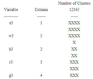Figure 6. The icicle plot according to the third eigenvalue of each of five organisms

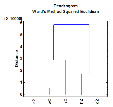
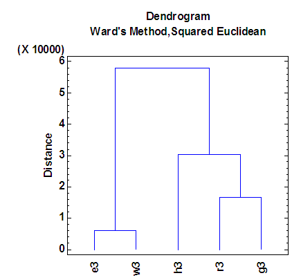Figure 7. Dendrogram according to the third eigenvalue of each of five organisms

It is clear that the clustering process based on the third eigenvalue differ, from the connection aspect, compared with clustering process based on the first and second eigenvalues.

3.4. For the Fourth Eigenvalue

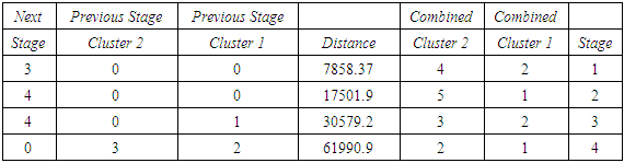
The agglomeration schedule in table (5), shows which variables were combined at each stage of the clustering process. For example, in the first stage, variable 2 was combined with variable 4. The distance between the groups when combined was 7858.37. It also shows that the next stage at which this combined group was further combined with another cluster was stage 3.

Table (5). Agglomeration Schedule for the fourth eigenvalue of each of five organisms

As a result, cluster analysis based on the fourth eigenvalue shows that the first connection is between E. coli and Wheat. The second connection is between Human and Grasshopper. The third connection is between Human and Grasshopper from the first hand and Rat on the other. The fourth connection is between Human and Grasshopper and Rat from the first hand and E. coli and Wheat on the other. Table (5) and figures 8 and 9 explain what we stated above.

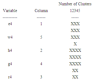Figure 8. The icicle plot according to the fourth eigenvalue of each of five organisms

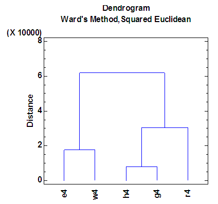Figure 9. Dendrogram according to the fourth eigenvalue of each of five organisms

It is clear that the clustering process based on the third eigenvalue differ, from the connection aspect, compared with clustering process based on the first, second and third eigenvalues.

We concluded that, the clustering process is different relatively depending on each one of the eigenvalues to the other, both in terms of the connection or in terms of distances values calculated for this purpose. This is a source of power of this research, as it will increase the necessary tests to distinguish between organisms according to the criteria under consideration and then increase the robustness of decision.

As further studies in future and next related research, another empirical studies should be done for other organisms and statistical methods by using the point of view adopted here. In addition, aspects stated here must be used for applied situations for DNA sequences discrimination.