1. Introduction

With rapid developments of financial markets in China, more and more futures contracts and financial derivatives have been listed on the four Chinese futures exchanges. Both the number of contracts and trade volumes have increased dramatically. The futures markets, together with other derivatives, play a more important role in Chinese financial markets providing various institutional and individual investors a convenient way of hedging risk or expressing their certain views on the market. However, the increasing scale of futures trading poses a challenge for the quantitative risk management within Chinese futures exchanges. With more contracts to trade, investors usually trade more than single contracts and they find that most of time their positions can cancel some degree of risk within their portfolio so that they demand decreasing charges of their risk margins from the exchanges. With a lower charge of risk margins, investors can trade more contracts and increase the efficiency of their funds. From the perspectives of financial exchanges, they expect that they can charge as less as possible risk margins for each investors while still keeping enough risk margins, so as to increase trade volumes and expand their businesses. For exchanges to accomplish this challenging task, it is very necessary for them to be equipped with a powerfully accurate statistical model to measure and predict the risk measures for all positions and portfolios of the investors. So this article has two purposes. First we like to illustrate how we can use a time-varying t copula framework to build a statistical forecasting model for quantitative risk management within Chinese futures exchanges. Secondly, by applying our model to intraday data of twelve main futures contracts traded on Shanghai Futures Exchange, we like to explore some empirical properties of price dynamics and dependence structures of commodity futures contracts traded on Chinese markets.

Copula has been frequently used in financial modelling for constructing joint distributions of multiple returns of financial assets. It provides practitioners with a more flexible way of finding the fittest dependence structures of multiple asset returns than just normal, t or other multivariate distributions. The special feature of copula is its capability of decomposing joint distributions of random variables into marginal distributions of individual variables and the copula which links the margins. With this feature, the task of finding a proper joint distribution becomes to find a copula form which features a proper dependence structure when marginal distributions of individual variables are properly specified. Among many copula candidates, t copula is a very good one, though not perfect, in terms of modeling joint distributions especially for a large number of asset returns. And t copula models are very useful tools to describe joint distributions of multiple assets for risk management and asset allocation purposes. In this paper, we show that how a time-varying t copula model can be easily applied to future price data and can reasonably well describe the dependence structure of multiple future returns.

We usually face two challenging issues when we apply copula theory to multiple time series. The first issue is about how to choose a copula function form that can best describe the data. As we know, different copulas feature different dependence structures between random variables. Some copulas may fit one particular aspect of the dataset very well but do not have a very good overall fit, while others may have the opposite performance. What criteria we should use when we choose from copula candidates is a major question remaining to be fully addressed. Secondly, how we can build a multivariate copula which is sufficiently flexible to simultaneously account for the dependence structure for each pair of random variables in the overall joint distribution is still quite challenging. We hope to shed some light on those two issues by applying our time-varying t copula model to the future price data.

In a copula model, we first model each asset return with a variant of GARCH specification. Based on different properties of each asset return, we choose a proper GARCH specification to formulate conditional distributions of each return. Then, we choose a proper copula function to link marginal distributions of each return to form the joint distribution. As in marginal distributions of each return, the copula parameters can also be specified as being dependent on previous observations to make the copula structure time-varying for a better fit of data. More specifically in this paper, we have an AR(1) process for the conditional mean and a GJR(1,1)¹ specification for the conditional volatility for each return. We employ a Student’s t copula with a time-varying correlation matrix (by a DCC specification²) to link marginal distributions. Usually the specified multivariate model contains a huge number of parameters and the estimation by maximum likelihood estimator (MLE) can be quite challenging. Therefore, we pursue a two-stage procedure, where the GARCH models for each return are estimated individually first and copula parameters are estimated in the second stage with estimated cumulative distribution functions from the first stage.

We apply our model to twelve log returns of twelve main future contracts traded on Shanghai Futures Exchange. The dataset spans from Jan 2, 2018 to December 28, 2018. We used ten-minute log returns which are calculated from the high frequency data we collected from trading front in one of the major Chinese futures brokers. Our estimation results show that the specification of AR(1) and GJR(1,1) with students’ t distribution can reasonably well capture empirical properties of individual future returns, which possess fat tails and leverage effects. We then estimate a DCC specification for the time-varying t copula. The parameter estimates of the time-varying t copula are statistically significant, which indicates a significant time-varying property of the dependence structure. For the twelve commodity future contracts, we find that the GARCH effects are statistically significant, while the leverage effects are not for some contracts. We also find that futures contract within the same categories or with close relations tend to have higher correlation and tail dependence behavior, while those without close relations tend to have quite low correlations and insignificant tail dependence behavior for ten-minute return data. The flexibility of t copula and its time-varying correlation structure significantly improve the model performance. As mentioned in the beginning, our t copula framework is very useful for risk management in future exchanges, specifically for Chinese futures exchanges with new future contracts and other financial derivatives such as options on futures.

This paper is organized as follows. Section 2 gives a short literature review on previous applications of copulas to modeling financial time series. Section 3 introduces our copula model where we introduce copula theory, t copula framework and estimation procedures. In particular, we elaborate on how to construct and estimate a time-varying t copula model. Section 4 documents data sources and descriptive statistics for Chinese futures data. Section 5 reports estimation results. Section 6 briefly discusses how our t copula framework can be applied to quantitative risk management in Chinese futures exchanges. Section 6 concludes.

2. Literature Review

Jondeau and Rockinger (2002) and Patton (2004, 2006a)³ proposed Copula-GARCH models to measure time-varying conditional dependence between time series. Jondeau and Rockinger (2002) use copula functions with time-varying parameters as functions of predetermined variables, and model marginal distributions with an autoregressive version of Hansen's (1994) GARCH-type model with time-varying skewness and kurtosis. They find for many market indices, dependency increases after large movements, more specifically, after extreme downturns. Patton (2006a) applies the Copula-GARCH model to modeling the conditional dependence between exchange rates and finds that Mark-dollar and Yen-dollar exchange rates are more correlated during depreciation against dollar than during appreciation periods. With a similar approach, Patton (2004) models the asymmetric dependence between "large cap" and "small cap" indices and examines the economic and statistical significance of the asymmetries for asset allocations in an out-of-sample setting. As in above literature, copulas are mostly used to capture asymmetric dependence and tail dependence between times series. For example, Gumbel's copula features higher dependence (correlation) at upper side with positive upper tail dependence and Rotated Gumbel's copula features higher dependence (correlation) at lower side with positive lower tail dependence. Hu (2006) studies the dependence structure between a number of pairs of major market indices by a mixed copula approach. Her copula is constructed by a weighted sum of three copulas-normal, Gumbel's and rotated Gumbel's copulas. Jondeau and Rockinger (2006) models the bivariate dependence between major stock indices by a Student’s t copula where the parameters are assumed to be modeled by a two-state Markov process.

The task of flexibly modeling dependence structure becomes more challenging for n-dimensional distributions. Savu and Trede (2006) develop a hierarchical Archimedean copula which renders more flexible parameters to characterize dependency between each pair of variables. In their model, each pair of closely related random variables is modeled by a copula of a particular Archimedean class and then these pairs are nested by copulas as well. The nice property of Archimedean family easily leads to the validity of the joint distribution constructed by this hierarchical structure. Tsafack (2006) builds up a complex multivariate copula to model four international assets (two international equities and two bonds). In his model, he assumes that the copula form has a regime-switching setup where in one regime he uses a n-dimensional normal copula and in the other he uses a mixed copula of which each copula component features the dependence structure of two pairs of variables. Zimmer and Trivedi (2006) apply trivariate hierachical Archimedean copulas to model sample selection and treatment effects with applications to the family health care demand.

Statistical goodness-of-fit tests can provide some guidance for selecting copula models. Chen et al. (2004) propose two simple goodness-of-fit tests for multivariate copula models, both of which are based on multivariate probability integral transform and kernel density estimation. One test is consistent but requires the estimation of the multivariate density function hence is suitable for a small number of random variables, while the other may not be consistent but requires only kernel estimation of a univariate density function, hence is suitable for a large number of assets. Berg and Bakken (2006) propose a consistent goodness-of-fit test for copulas based on the probability integral transform and they incorporate in their test a weighting functionality which can increase influence of some specific areas of copulas.

Due to their parameter structure, the estimation of copula-GARCH models also suffers from "the curse of dimensionality"⁴. The exact maximum likelihood estimator (MLE) works in theory⁵. In practice, however, as the number of time series being modeled increases, the numerical optimization problem in MLE will become formidable. Joe and Xu (1996) propose a two-stage procedure, where in the first stage only parameters in marginal distributions are estimated by MLE and then the copula parameters are estimated by MLE in the second stage. This two-stage method is called inference for the margins (IFM) method. Joe (1997) shows that under regular conditions the IFM estimator is consistent and has the property of asymptotic normality and Patton (2006b) also shows similar estimator properties for the two-stage method. Instead of estimating parametric marginal distributions in the IFM method, we can estimate the margins by using empirical distributions, which can avoid the problem of mis-specifying marginal distributions. This method is called Canonical Maximum Likelihood (CML) method by Cherubini et al. (2004). Hu (2006) uses this method and she names it as a semi-parametric method. Based on Genest et al. (1995), she shows that CML estimator is consistent and has asymptotical normality. Moreover, copula models can also be estimated under a non-parametric framework. Deheuvels (1981) introduces the notion of empirical copula and shows that the empirical copula converges uniformly to the underlying true copula. Finally, Xu (2004) shows how the copula models can be estimated with a Bayesian approach. The author shows how a Bayesian approach can be used to account for estimation uncertainty in portfolio optimization based on a Copula-GARCH model and she proposes to use a Bayesian MCMC algorithm to jointly estimate the copula models.

Much research has been done to describe the dynamics of commodity future prices using GARCH models. With respect to univariate future price, researchers apply a variety of GARCH specifications to forecasting conditional distributions (mainly volatility) of future prices. Yang et al. (2001) study the effect of radical agricultural liberalization policy in 1996 on agricultural commodity price volatility using GARCH models; Hung et al. (2008) investigate the influence of fat-tailed innovations on the performance of one-day-ahead VaR estimates for energy commodity futures using GARCH models. Some recent papers include Kristjanpoller and Minutolo (2016), Nguyen and Walther (2018), and Čermák et al. (2017). For multiple future prices, research has been mainly focused on the issues of optimal hedging ratios and risk management. See, for example, Baillie and Myers (1991) and Zhang and Choudhry (2015).

3. The Model

3.1. Copula

We introduce our copula model by first introducing the concept of copula. A copula is a multivariate distribution function with uniform marginal distributions as its arguments, and its functional form links all the margins to form a joint distribution of multiple random variables⁶. Copula theory is mainly based on the work of Sklar (1959) and we state the Sklar's theorem for continuous marginal distributions as follows.

Theorem 1 Let be given marginal distribution functions and continuous in respectively. Let H be the joint distribution of . Then there exists a unique copula C such that

(1)

Conversely, if we let be continuous marginal distribution functions and C be a copula, then the function H defined by Equation (1) is a joint distribution function with marginal distributions .

The above theory allows us to decompose a multivariate distribution function into marginal distributions of each random variable and the copula form linking the margins. Conversely, it also implies that to construct a multivariate distribution, we can first find a proper marginal distribution for each random variable, and then obtain a proper copula form to link the margins. Depending on which dependence measure used, the copula function mainly, not exclusively, governs the dependence structure between individual variables. Hence, after specifying marginal distributions of each variable, the task of building a multivariate distribution solely becomes to choose a proper copula form which best describes the dependence structure between variables.

Differentiating equation (1) with respect to leads to the joint density function of random variables in terms of copula density. It is given as

(2)

where is the copula density and is the density function for variable i. Equation (2) implies that the log-likelihood of the joint density can be decomposed into components which only involve each marginal density and a component which involves copula parameters. It provides a convenient structure for a two-stage estimation, which will be illustrated in details in following sections.

To better fit the data, we usually assume the moments of distributions of random variables are time-varying and depend on past variables. Therefore, the distribution of random variables at time t becomes a conditional one and then the above copula theory needs to be extended to a conditional case. It is given as follows⁷.

Theorem 2 Let be the information set up to time t and let be continuous marginal distribution functions conditional on . Let H be the joint distribution of conditional on . Then there exists a unique copula C such that

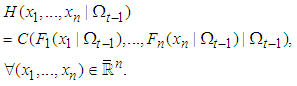(3)

Conversely, if we let be continuous conditional marginal distribution functions and C be a copula, then the function H defined by Equation (3) is a conditional joint distribution function with conditional marginal distributions .

It is worth noting that for the above theorem to hold, the information set has to be the same for the copulas and all the marginal distributions. If different information sets are used, the conditional copula form on the right side of (3) may not be a valid distribution. Generally, the same information set used may not be relevant for each marginal distributions and the copula. For example, the marginal distributions or the copula may be only conditional on a subset of the universally used information set. At the very beginning of estimation of the conditional distributions, however, we should use the same information set based on which we can test for insignificant explanatory variables so as to stick to a relevant subset for each marginal.

3.2. Modeling Marginal Distributions

Before building a copula model, we need to find a proper specification for marginal distributions of individual asset returns, as mis-specified marginal distributions automatically lead to a mis-specified joint distribution. Let be asset i’s return at time t and its conditional mean and variance are modeled as follows.

(4)

(5)

(6)

As shown in equations (4) to (6), we model the conditional mean as a AR(1) process and the conditional variance as a GJR(1,1) specification⁸. We have parameter restrictions as , , , and 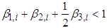. is an indicator function, which equals one when and zero otherwise. We believe that our model specifications can capture the features of the individual stock returns reasonably well. It is worth noting that equations (4) to (6) can include more exogenous variables to better describe the data. Alternative GARCH specifications can be used to describe the time-varying conditional volatility. We assume is across time and follows a Student’s t distribution with DoF (degree of freedom).

Alternatively, to model the conditional higher moments of the series, we can follow Hansen (1994) and Jondeau and Rockinger (2003) who assume a skewed t distribution for the innovation terms of GARCH specifications and find that the skewed t distribution fits financial time series better than normal distribution. Accordingly, we can assume 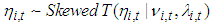with zero mean and unitary variance where is DoF parameter and is skewness parameter. The two parameters are time-varying and depend on lagged values of explanatory variables in a nonlinear form. For illustration purposes, however, we will only use Student’s t distribution for in this paper.

3.3. Modeling Dependence Structure

Normal copula and Student's t copula are two copula functions from elliptical families, which are frequently used in modeling joint distributions of random variables. In this chapter, we also estimate a normal copula model for comparison purposes. Let denote the inverse of the standard normal distribution and be n-dimensional normal distribution with correlation matrix. Hence, the n-dimensional normal copula is

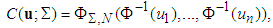(7)

and its density form is

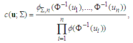(8)

where and are the probability density functions (pdf’s) of and respectively. It can be shown via Sklar's theorem that normal copula generates standard joint normal distribution if and only if the margins are standard normal.

On the other hand, let be the inverse of standard Student's t distribution with DoF parameter⁹ and be n-dimensional Student's t distribution with correlation matrix R and DoF parameter v. Then n-dimensional Student's t copula is

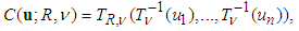(9)

and its density function is

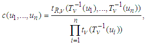(10)

whereand are the pdf’s of and respectively.

Borrowing from the dynamic conditional correlation (DCC) structure of multivariate GARCH models, we can specify a time-varying parameter structure in the t copula as follows¹⁰. For a t copula, the time-varying correlation matrix is governed by

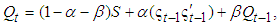(11)

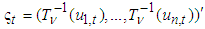
where S is the unconditional covariance matrix of , and and are non-negative and satisfy the condition . We assign and the dynamics of is given by (11). Let be the element of the matrix and the element of the conditional correlation matrix can be calculated as

(12)

Moreover, the specification of (11) guarantees that the conditional correlation matrix is positive definite.

Proposition 1 In equations (11) to (12), if

and ,

all eigenvalues of S are strictly positive,

then the correlation matrix is positive definite.

Proof: First, a) and b) guarantee the system for is stationary and S exists. With , c) guarantees is positive definite. With a) to c), is the sum of apositive definite matrix, a positive semi-definite matrix and a positive definite matrix both with non-negative coefficients, and then is positive definite for all t. Based on the proposition 1 in Engle & Sheppard (2001), we prove that is positive definite.

3.4. Estimation

We illustrate the estimation procedure by writing out the log-likelihoods for observations. Let be the set of parameters in the joint distribution where is the set of parameters in the copula and is the set of parameters in marginal distributions for asset i. Then the conditional cumulative distribution function (cdf) of n asset returns at time t is given as

(13)

where is a vector of previous observations, is the conditional copula and is the conditional cdf of the margins. Differentiating both sides with respect to leads to the density function as

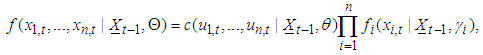(14)

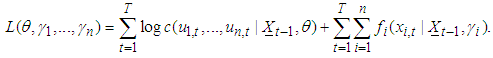
where is the density of the conditional copula and is the conditional density of the margins. Accordingly, the log-likelihood of the sample is given by

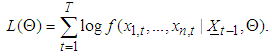(15)

With equation (15), the log-likelihood can be written as

(16)

From equation (16), we observe that the copula and marginal distributions are additively separate. Therefore, we can estimate the model by a two-stage MLE procedure. In the first stage, the marginal distribution parameters for each asset are estimated by MLE and then with estimated cdf of each asset, we estimate the copula parameters by MLE. Based on Joe (1997) and Patton (2006b), this two-stage estimator is consistent and asymptotically normal.

With our model specifications, we first estimate the univariate GJR-GARCH(1,1) with an AR(1) conditional mean and Student’s t distribution by MLE. In the second stage, we need to estimate the parameters for the constant normal copula and the time-varying Student’s t copula. Let , and we can analytically derive the correlation matrix estimator which maximizes the log-likelihood of the normal copula density as

(17)

As there is no analytical solution for MLE of Student's t copula, the numerical maximization problem is quite challenging. Following Chen et al. (2004), however, with we can calculate the sample covariance matrix of as , which is a function of DoF parameter . By setting , we can express and for all t in terms of , and using equation (11). Then we can estimate , and by maximizing the log-likelihood of t copula density. In the following sections, we apply our estimation procedure to the joint distribution of 45 selected major U.S. stock returns.

4. Data

We apply our model to the log returns of twelve commodity future contracts traded on Shanghai Futures Exchange¹¹. Table 1 shows future contract symbols, trade unit, quote unit, minimum price change and trading time. The data set spans from Jan 2, 2018 to December 28, 2018. We first collect high frequency data from trading front through one of the major Chinese futures brokers and then calculate the ten-minute log returns¹² of future prices based on the collected high frequency data. The original data we collected have a frequency of half second and in some cases when there is no new market activity then we will not receive any data feed from the exchange. The price we use for calculating log returns are middle price which is the average of buy and sell prices. Since every future contract will expire, we construct our prices series by connecting prices of all the main contracts for each commodity. Main contracts are defined as the contracts with maximum open interests. Moreover, as the twelve future contracts have different trading time periods during the night, we only include the time periods where all contracts are traded (21:00-23:00) during the night in our analysis. When price series shift from one contract to another due change of main contract or include non-trading periods, the absolute value of calculated log returns can be extremely large. Therefore, we assign the price change to zero when main contracts change or trading stops.

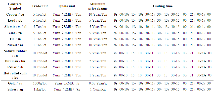Table 1. This table shows the trade unit, quote unit, minimum price change and trading time for twelve futures contracts traded on Shanghai Futures Exchange

We first plot ten-minute log returns of twelve commodity futures in Figure 1. We observe that log returns fluctuate around zero and have clusters of volatility. Even when we exclude the outlier from change of major contracts or non-trading periods, we still have some outliers during trading periods. Table 2 shows the calculated mean, standard deviation, skewness and kurtosis for the twelve contracts. We observe that all contracts have almost zero means. Rubber, rebar, bitumen, zinc and hot rolled coils have relatively higher standard deviations. Most contracts have slightly positive skewness while rubber, copper and tin have slightly negative skewness. More importantly, all the commodities have kurtosis higher than three, which implies fat tails. All those observations indicate that we should use a GARCH-type model to fit the data and account for clusters of volatility and fat tails.

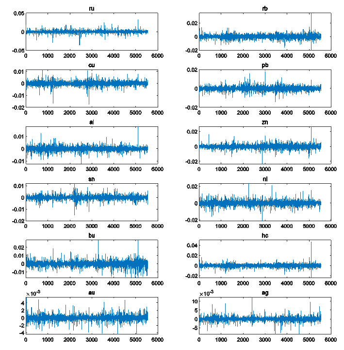Figure 1. This figure shows the ten-minute log returns of twelve major futures prices traded on Shanghai Futures Exchange

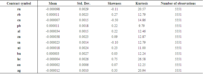Table 2. This table shows descriptive statistics (mean, standard deviation, skewness and kurtosis) for the twelve commodity future contracts

5. Empirical Results

5.1. Marginal Distributions

We briefly report estimation results for marginal distributions of twelve futures contracts. Table 3 shows the estimates and t statistics for estimation of parameters in the specifications of conditional mean and conditional variance. For conditional mean, we find that except zinc (zn) and nickel (ni), all other contracts have t statistics greater than two, which indicates statistically nonzero parameters at the first lag. For conditional variance, we find that parameters for constants, GARCH and ARCH components, and DoF are statistically nonzero for almost all the contracts. It is worth noting, however, that for nine out of twelve contracts, the parameters for leverage effects are not statistically significant, which indicates GARCH(1,1) might be a better choice than GJR(1,1) for those contracts¹³. In summary, the log returns of future prices at ten-minute intervals have significant GARCH effects for all the contracts but no significant leverage effects for many future contracts. Moreover, all the futures contracts have fat tails. In figure 2 we plot the estimated conditional variances for all the contracts and observe that all contracts have clusters of volatility and volatility spikes. This observation indicates that the log returns of future contracts at ten-minute intervals possess significant degree of market risk, which is worthwhile for practitioners to seriously consider for intraday risk management.

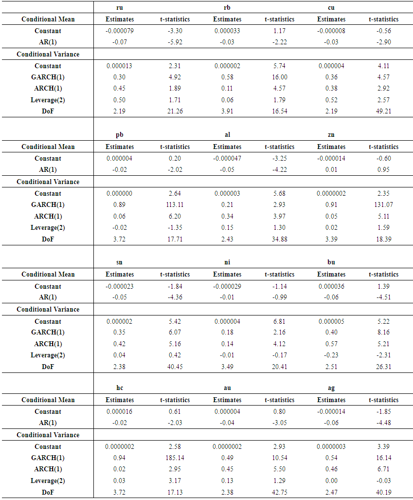Table 3. This table shows the estimation results of the conditional mean and conditional variance for the twelve future contracts

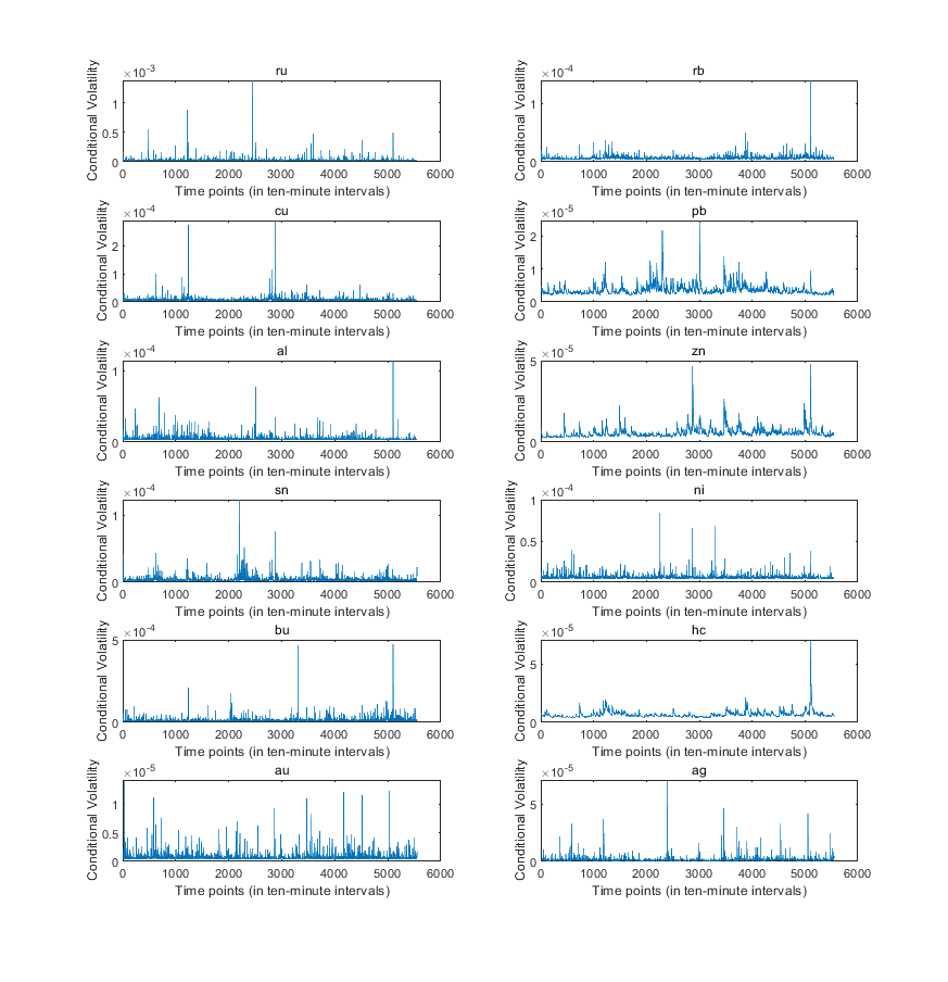Figure 2. This figure shows the plots of estimated conditional volatility for the twelve future contracts

5.2. Copulas

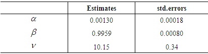
In table 4, we report estimation results for the parameters of time-varying t copula. All the three parameters , and are statistically nonzero based on the reported standard errors. The estimate is close to zero and the estimate for is close to one. The estimate for is about 10. As our estimation is carried out on the joint distribution of twelve future returns, the estimate for shed some light on how much Student’s t copula can capture tail dependence when used to fit a number of variables. Previous research shows that the time-varying Student’s t copula leads to significant higher log-likelihood than normal copula when applied to the same data set¹⁴. This results from the more flexible parameter structure of t copula and the time-varying parameter structure.

Table 4. This table shows the estimates and standard errors for time-varying Student’s t copula

5.3. Time-varying Dependence

Our time-varying t copula features a time-varying dependence structure for all the variables. The DoF parameter, together with the correlation parameters, governs the tail dependence behavior of multiple variables. We plot the estimated conditional correlation parameters of t copula for sex selected pairs of futures returns in Figure 3. For those six pairs, the conditional correlation parameter fluctuates around certain positive averages. We purposely select the first three pairs, rubber and hot rolled coils, gold and silver, and copper and nickel, and those pairs are either in the same categories of commodity or belong to close categories. Therefore, we find their correlations parameters are all greater than 0.5. For the other three pairs, copper and tin, tin and silver, and rubber and bitumen, they belong to different categories of commodities. Accordingly, we find their correlation parameters are quite low. Moreover, we plot the estimated TDCs (tail dependence coefficients) for the 6 selected pairs of future contracts. Consistent with plots of correlations, we find that for the first three pairs, TDCs are relatively higher than the other three pairs. Specifically, TDCs for the pairs of rubber and hot rolled coils, gold and silver, and copper and nickel are around 0.5, 0.2 and 0.2. For the last three pairs which do not belong to the same categories, TDCs are only around 0.05, 0.02 and 0.05. We can conclude from the plotted dependence measures our model can account for the time-varying dependence structures of future contracts reasonably well.

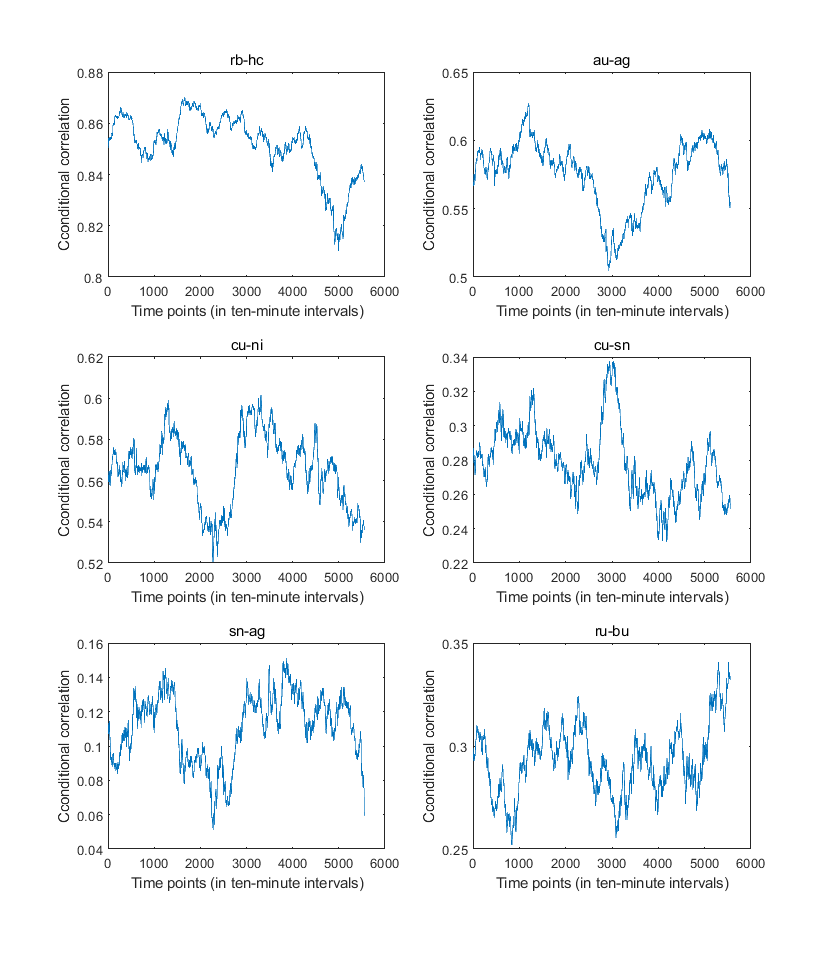Figure 3. This figure plots the estimated time-varying correlation parameters in t copula for the selected 6 pairs of future contracts

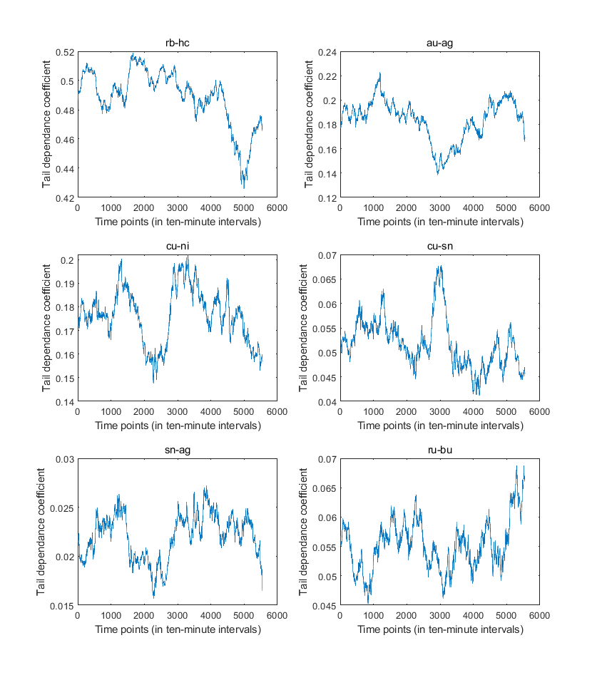Figure 4. This figure plots the estimated TDCs (tail dependence coefficients) for the selected 6 pairs of future contracts

6. Applications of t Copula Models for Quantitative Risk Management in Chinese Futures Exchanges

In this section, we briefly illustrate how a futures exchange can build up a quantitative framework for better forecasting risk measures for investors’ trading accounts using time-varying t copula models. Specifically, as the number of futures contracts and other financial derivatives increases in major Chinese futures exchanges, it becomes more and more relevant to have a quantitative framework which can more accurately generate risk measures for all trading accounts of investors for different time horizons. We believe our time-varying t copula model can do this task sufficiently well. Let’s take Shanghai Futures Exchange as an example. There are currently fourteen commodity futures and one option on commodity futures traded on Shanghai Futures Exchange. Those fourteen commodity futures have their multiple contracts with different expiration dates. The options are based on the prices of one commodity future with multiple contracts of different expiration dates.

We first need to decide on underlying risk factors on which all the financial instruments traded are based. For the fourteen commodity futures, we would use the major contracts for each commodity and for each commodity we can add certain adjustments for other expiration dates¹⁵. Because the options are also based on commodity futures, we use the time-varying t copula model to model the joint distributions of fourteen major commodity futures.¹⁶ With time-varying t copula model, together with the adjustment specification for contracts with other expiration dates, we can forecast the joint distributions of log returns of all the currently traded future contracts. With this joint distribution, we can forecast by Monte Carlo simulations the risk measures of different portfolios including various combinations of financial instruments.

It is worth pointing out that we can construct the time-varying t copula framework to forecast the risk measures for different time horizons. The forecast time horizon can be weekly, daily or hourly. With forecasts of risk measures for all the financial portfolios at a range of horizons, the exchange can possess a compressive view on the future risk of trading accounts of their clients and this will provide the exchange more accurate and confidant suggestions when dealing with all risk management operations.

7. Conclusions

In this paper, we illustrate how to model and forecast the joint distribution of multiple returns of futures prices by a time-varying Student’s t copula model and how this model framework can be applied to the twelve major future contracts traded on Shanghai Futures Exchange. We model the ten-minute log returns of future prices for the year of 2018 and find that the specification of AR (1) and GJR (1,1) can fit the individual return series reasonably well and the time-varying t copula with a DCC specification can more flexibly describe the dependence structure and significantly improve the fitness of the data. For the twelve commodity future contracts, we find that the GARCH effects are statistically significant, while the leverage effects are not for some contracts. We also find that futures contract within the same categories or with close relations tend to have higher correlation and tail dependence behavior, while those without close relations tend to have quite low correlations and insignificant tail dependence behavior for ten-minute return data.

We also briefly illustrate how our model can be applied to the quantitative risk management in Chinese futures exchanges. We show that our model can be effectively used to forecast the joint distribution of all the underlying risk factors on which all financial instruments are traded and priced, and to calculate risk measures of different combinations of instruments in different investors’ accounts for different time horizons.

As it is quite challenging to find a copula function with very flexible parameter structure to account for difference dependence features among all pairs of random variables, our time-varying t copula model tends to be a good working tool to model multiple asset returns for risk management and asset allocation purposes. Our model can capture time-varying conditional correlation and some degree of tail dependence, while it also has limitations of featuring symmetric dependence and inability of generating high tail dependence when being used to model a large number of asset returns. Nevertheless, we hope that this framework can effectively serve as practical tools for risk management at Chinese futures exchanges and leave that above limitations for future research.

^#This research project is supported by Shanghai Pujiang Talent Program (project code: 14PJC066).

Notes

1. See section 3.2 and Glosten et al. (1993) for details.

2. See section 3.3 and see Engle and Sheppard (2001) and Engle (2002) for details.

3. Alternative approaches are also developed, such as in Ang and Bekaert (2002), Goeij and Marquering (2004) and Lee and Long (2006), to address non-normal joint distributions of asset returns.

4. For a detailed survey on the estimation of Copula-GARCH model, see Chapter 5 of Cherubini et al. (2004).

5. See Hamilton (1994) and Greene (2003) for more details on maximum likelihood estimation.

6. See Nelsen (1998) and Joe (1997) for a formal treatment of copula theory, and Bouye et al. (2000), Cherubini et al. (2004) and Embrechts et al. (2002) for applications of copula theory in finance.

7. See Patton (2004).

8. See Glosten et al. (1993).

9. In contrast to the previous standardized Student’s t distribution, the standard Student’s t distribution here has variance as v/(v - 2).

10. Please see Engle and Sheppard (2001) and Engle (2002) for details on the multivariate DCC-GARCH models.

11. There are all together 14 commodity futures traded on Shanghai Futures Exchange. They are natural rubber (ru), lead (pb), aluminum (al), copper (cu), zinc (zn), tin (sn), nickel (ni), bitumen (bu), rebar (rb), hot rolled coils (hc), gold (au), silver (ag), wire rod (wr) and fuel oil (fu). As wire rod and fuel oil suffer from either an insufficient trading volume or a short trading history, we exclude those two contracts from our analysis.

12. Log returns are defined as the first difference of the natural logarithm of the prices. In our case we take first difference of logarithm of prices at ten-minute intervals.

13. In practice, one may use GARCH(1,1) to replace GJR(1,1) for possibly better fitness of the data. Without much risk of model misspecification, however, we still use GJR(1,1) in our paper for convenience.

14. Kang (2015) applied the same model to 45 U.S. stock returns and shows that time-varying t copula model leads to significant higher log-likelihood than normal copula model.

15. We only illustrate the ideas here and will not provide the detailed specifications for the adjustments.

16. We can use t copula model to model the joint distribution of those fourteen log returns of major contracts. We can add certain adjustments to the major contracts to derive the distribution of contracts with other expirations.