1. Introduction

Financial markets exhibit certain regularities in what has become known in the literature as stylized facts. Certain findings seem to occur with some regularity that it has come to be accepted as a matter of course. However, statistical models which seek to uncover the behaviour of financial variables has for long given mixed results when applied to different market settings. One such model, so central to finance and economics, is the volatility model used to estimate the heteroscedasticity of a financial time series. Volatility is ubiquitous in finance. It plays a major role in the pricing of financial instruments, trading, managing and monitoring of risk. As a concept, its latent nature means it can only be estimated from historical data and then forecast forwards. Estimating volatility has been challenging throughout finance and economics literature spawning numerous models to capture various aspects of it through time. Starting with the pioneering work of Engle [1] on autoregressive conditional heteroscedastic (ARCH) model for estimating volatility in inflation data of the United Kingdom, research has since exploded with researchers tinkling with various models based on the generalised autoregressive conditional heteroscedasticity (GARCH) developed by Bollerslev [2].

Among many variants, Nelson [3] proposed the exponential GARCH to account for the so-called leverage effect in volatility dynamics. Past negative observations tend to have a larger effect on the conditional volatility compared with past positive returns of similar magnitude. This important observation was earlier reported in the literature by Black [4] and Christie [5]. Similarly, Glosten et al. [6] proposed a model that captured the asymmetry induced by negative shocks to the conditional volatility process. Majority of these models nest the GARCH. Zakoian [7] introduced the threshold GARCH (TGARCH) which does not nest the GARCH. The TGARCH differs from the other GARCH models in the way it uses standard deviation instead of variance in the modeling process. For a review of GARCH models and their applications see Xu et al. [8], Teräsvirta [9], Bauwens et al. [10], Brooks et al. [11], Poon and Granger [12] and Hentschel [13].

There are important shortcomings of GARCH, however. The accuracy of calculations and forecasts of volatility for nonlinear data using GARCH models have been the subject of continuing research and criticism [14]. This could be due to the very basic assumption underpinning GARCH models. GARCH family of models assumes deterministic volatility states. However, it is known that volatility itself can be taken as a stochastic variable. This gave rise to the adoption of models that assume the stochasticity of the volatility states. In the stochastic volatility (SV) paradigm, we remove the restrictions on the model parameters, a difficulty in GARCH-type estimation. More importantly, both the return equation and the volatility model are driven by separate innovative process. This makes SV models flexible and are able to capture the characteristics of the volatility in the returns.

In this paper, we provided a Bayesian implementation of the volatility of the returns of the Ghana Stock Exchange All Share index (henceforth GSE index) within both the framework of stochastic volatility and GARCH(1,1) with student's t innovations. Both models have been implemented using Bayesian statistics in order to have a uniform set of statistics as a basis for comparison.

Our findings are two-fold. First we found that even for a large data set, the parameter estimates differ in both paradigms of volatility modeling. This result is consistent with findings in empirical finance of both the GARCH(1,1) and SV models giving different estimates of volatility parameters. We also found that for the period under review, the GARCH(1,1) seems adequate in terms of parsimony and model fit compared to the SV model. This is very much at odds with findings and recommendations in finance [15]. We think it may be due to the developmental stage of the particular market in question. This, in our view, warrants further research in markets with similar characteristics as that of the GSE.

This paper is novel in one important aspect. It is the first, to the best knowledge of the authors, to incorporate Bayesian methodology in volatility estimation for both GARCH(1,1) and SV frameworks in modeling the volatility of the returns of the GSE index. This approach has been shown by Ghysels et al. [16] and Jacquier, Polson and Rossi [17] to be parsimonious. There is a plethora of papers on modeling volatility of returns of the GSE index; see Boako et al. [18], Frimpong and Oteng-Abayie [19] and Alagidede and Panagiotidis [20]. All these papers used GARCH class models. This research therefore should be seen as a departure from these approaches in adopting a Bayesian framework. Bayesian methods offer a natural solution to the generality of volatility modeling problems where we estimate parameters using own lag values. There could be other drivers of risk that are latent; thus escaping specification and/or accurate measurement. This transforms an otherwise deterministic problem into a stochastic one with consequences for the model. The Bayesian paradigm can therefore be seen as incorporation model uncertainty due to measurement errors, model misspecification and omitting variables.

The rest of the paper is organised as follows. Section 2 reviews the literature on GARCH, SV and the Bayesian modeling approach. The mathematical representation of the stochastic volatility and GARCH model is given in section 3. This mathematical representation relies on the Bayesian method of estimating model parameters. Section 4 is therefore on the prior estimation for the Bayesian posterior estimation. Section 5 looks at data analysis, results and discussion. This includes model comparison of SV with the GARCH(1,1). Finally section 6 concludes the paper.

2. Literature

(G)ARCH models were the first serious attempts at modeling time-varying conditional heteroscedasticity. Engle's [1] original idea of the ARCH models was to linearly regress the time t variance of the process on the p squared errors from prior time periods. This idea was a departure from the constant variance in vogue at the time. It was appealing intuitively and so it quickly gained traction among academics and finance practitioners. However, model parsimony was a problem. ARCH models required long lags into the past. It also has the limitation of being unable to deal with asymmetric and leverage effects in volatility. To deal with the first limitation, Bollerslev [2] proposed, in addition to the p lagged square errors, to include lagged values of the variance. This serves to make the GARCH model parsimonious. The model is also able to describe a wide range of behaviours that characterise volatility of returns empirically.

SV models provide an alternative to GARCH models. Fundamentally, GARCH models have one source of variation which is the innovations z_t distributed as iid N(0,σ_ε²). The expectation and variance of the innovations is deterministic. There is a single white noise process driving both the conditional mean and the conditional volatility. This does not allow for any variation in the error process of the volatility dynamics. This is clearly at variance with the empirical behaviour of volatility in financial time series. Additionally, GARCH models are subject to a number of constraints to ensure a positive variance. As Nelson [3] noted, these constraints are violated during the process of estimating the GARCH parameters.

In observed financial times series, volatility clusters characterise returns. These clusters are observed to be time-varying too. This suggests to account for the random variation in the conditional expectation and the conditional variation separately. This is the idea of SV models. Unfortunately, SV modeling presents a difficulty. Instead of one, an additional error process has to be taken into account in modelling. This calls for Bayesian approaches. References to the use of Bayesian methods in volatility modeling go back to the work of Jeffrey [21] with the use of Jeffrey priors in significance testing. It was established then that the volatility of financial returns varies randomly with time. Clark [22] also documented this observation in an early attempt at giving a mathematical form to the variation in speculative futures. He proposed a mixture of distributions for the returns on stocks. An early application was by Taylor [23] who formalised the concept in a statistical form. He modelled the volatility of sugar prices by explicitly modelling the randomness of the conditional mean and conditional variance separately with the logarithm of the variance following an autoregressive process. In short SV is modelled to capture the heteroscedasticity of the volatility process by having its own set of innovations or shocks. Since then, there has been a plethora of papers extending SV in all areas of finance and economics. This has been made possible largely by the adoption of numerical techniques of analysis in solving computationally intractable problems using efficient Markov chain Monte Carlo (MCMC) methods for sampling posterior distributions. This has been made possible by advances in Bayesian statistics over the last three decades. Bayesian methods are parsimonious and give outputs that are easily interpretable. The concept has been particularly used in the pricing of derivatives where risk modeling is of utmost importance.

Andersen [24] extended stochastic volatility and provided a general framework for autoregressive modeling of the volatility of financial time series. Since then, numerous researchers have found various paths for applying this framework in finance and economics. They have found use particularly in the area of option pricing where volatility of the return on assets is a key input [25-28]. Hobson and Rogers [29], Renault and Touzi [30] and Andersen and Andreasen [31] explained the phenomenon of volatility smile surface in implied volatility using SV. SV has provided the tools to model jumps in financial data at multiscale [32]. In areas as varied as high frequency volatility modeling, jumps are a frequent feature and very difficult to capture. Busch et al [33] employed SV to capture these discontinuities in the foreign exchange, bond and stock markets. It has also been used in coming up with new types of risks in the finance industry [34].

3. The Models

3.1. Stochastic Volatility

We adopt the notation of Kastner [35] in specifying the stochastic volatility model. Consider a vector of return series which have been demeaned. The SV is stated in hierarchical form as:

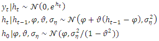where is a normal distribution with mean μ and variance . The vector of parameters

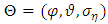where μ is the level of log-variance, φ is the persistence of log-variance and the volatility of log-variance is are to be estimated. The process 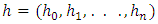is the latent conditional volatility process with the as the initial stationary autoregressive process of order one.

3.2. GARCH(1,1)

Consider a stationary series given by . The returns relation is stated as

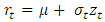with being the student's t-innovations with degrees of freedom. The GARCH(1,1) model is specified as:

with the restriction on the parameters and . The parameters are to be estimated using the Bayesian sampling method.

4. Prior Estimation

Bayesian methods involve an integral which sometimes no analytic solution. A numerical method involving a Markov chain Monte Carlo algorithm offers a powerful and intuitive framework for solving flexibly the integration numerically. This has been made possible by the advent of low cost computing technology and efficient MCMC samplers. We use the random walk Metropolis-Hasting algorithm of the MCMC to construct the Markov-chain simulation of the posterior. We need to specify the prior and likelihood as the basis for estimating the posterior. From the posterior, we draw inferences about our volatility parameters.

Choosing our priors for the problem relies on the recommendations set out in Kim et al. [36]. The prior consists of independent hyperparameters whose joint distributions is stated as a product given the parameter space as:

with the parameters previously defined. , the level of log-variance, is taken to be a normal prior . This prior is chosen to be noninformative ie. and . This is to allow the likelihood to contain most of the information. We chose a beta function with parameters for the persistent parameter with to ensure the stationarity of the autoregressive volatility of the process . The beta distribution is thus given as 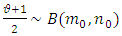with the density function expressed as:

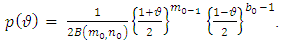The expectation and variance of this distribution is given respectively as:

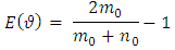and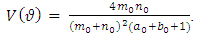

Suggestions for the choices of and are made in Kim et al. [36]. For the choice of the distribution of the of the volatility of log-variance , we follow the recommendations of Frühwirth-Schnatter and Wagner [37] who selected so that

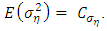
5. Data and Analysis

We obtained the daily closing indices of the GSE All-Share Index for the period from January 04, 2011 to March 31, 2017 giving 1549 data points. We calculated the log-returns from where is the price at time t to obtain a total of 1548 data points.

5.1. Descriptive Statistics

A time series plot in Figure 1 shows how the level of the index has evolved on the years. The index peaked around January 2014 and remained at that level with marked fluctuations until about July 2015. The market calmed thereafter with the level fluctuating around a downward trend until January 2017 when it bottomed up.

Figure 1. Time series of index levels of the GSE index

To make the series stationary, we took the differences of the logarithm prices to get the returns. A plot of the returns in Figure 2 shows apparent stationarity. There were extreme outcomes in the returns towards the end of 2015.

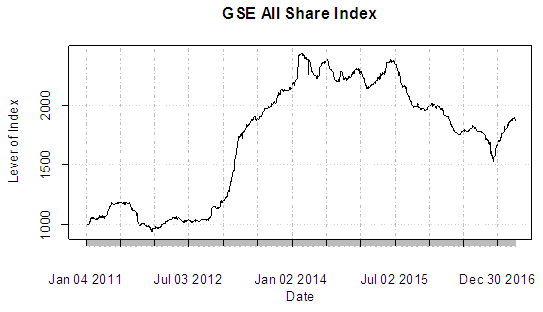
Figure 2. Time series of log-returns of the GSE index

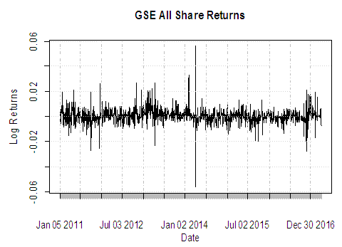
We conducted the augmented Dickey-Fuller test for the series. It yielded a ; hence we reject the null hypothesis of unit root at the 5% significance level and conclude that the series is stationary. A histogram of the returns is shown in Fig. 3. We superimposed the normal curve on the histogram. We can see that the distribution has fat tails.

Figure 3. Histogram of the log-returns of the GSE Index

A summary of the statistics of the returns is given in Table 1. The kurtosis confirms the presence of fat tails.

Table 1. Summary statistics of returns of GSE index

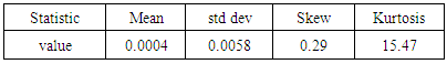
Engle's LM test for the presence of GARCH effects yielded a - statistic of 295.66 with a 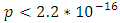confirming the presence of heteroscedasticity.

5.2. SV and GARCH(1,1)

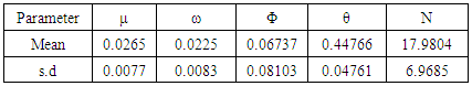
We estimated the models for the Bayesian SV and GARCH(1,1) using student-t innovations. Our choice of t-innovations was informed by the fat tailed distribution. The result of the parameters for the SV and GARCH(1,1) are displayed in Table 2 and 3 respectively.

Table 2. Posterior summary of the SV model

Table 3. Posterior summary of the GARCH(1,1) model

The penalised deviance of the SV and GARCH(1,1) are 1917 and 1897 respectively. This shows that the GARCH model fits the data better than the SV. Figure 4 compares the evolution of volatility of both models. It is seen that the SV model consistently over-estimates the volatility during the period.

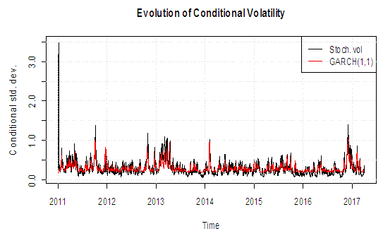Figure 4. Conditional volatility of log-returns estimated by the SV and the GARCH(1,1) models

6. Conclusions

Stochastic volatility models provide an alternative to the GARCH(p,q) models when estimating the parameters of the heteroscedastic process. In the developed markets, the SV has generally been found to be better in terms of model fit compared to the GARCH. This finding is across different asset classes. Frontier markets have their own idiosyncrasies which are clearly reflected in the statistics generated. Thin and asynchronous trading effects are two characteristics of trading in the relatively young markets. These effects influence the data generating process and give it different stylized effects. For example, the skew of the distribution of the return on the index was positive, a fact that has always been negative in developed markets. This may be due to the lack of crowding which leads to attractive valuations in frontier markets with above average returns.

We showed in this paper that GARCH(1,1) fits the data better than the SV model. SV consistently over-estimated the volatility for the period. Given the centrality of risk in finance, any model that over-estimates volatility will likely lead to mispricing with serious consequences for investors. For markets in their early stage of development, we still have to rely on the recommendation of Hansen and Lunde [38] who noted that nothing beats the GARCH(1,1).

ACKNOWLEDGEMENTS

The authors wish to thank Shiva G. Enchill of Bank of Ghana for kindly making the data available for this research.