Keran Song1, Zhengzheng Qian2
1Citigroup, Tampa, USA
2Department of Economics, Florida International University, Miami, USA
Correspondence to: Keran Song, Citigroup, Tampa, USA.
| Email: |  |
Copyright © 2017 Scientific & Academic Publishing. All Rights Reserved.
This work is licensed under the Creative Commons Attribution International License (CC BY).
http://creativecommons.org/licenses/by/4.0/

Abstract
We investigate the relationship between sectoral stock returns and the business cycle in three different ways. First, we calculate constant correlation coefficients between the business cycle and sectoral stock returns. Then, we employ the DCC GARCH model to estimate time-varying correlation coefficients for each pair of the business cycle and sectoral stock returns. Finally, we run regression of sectoral returns on dummy variables which are established according to four stages of the business cycle. All three sections reveal close relationships between sectoral stock returns and the business cycle. Some portfolio management suggestions are made last.
Keywords:
Sectoral stock returns, Business cycle, Correlation coefficient, Dynamic conditional correlation, Dummy variable regression
Cite this paper: Keran Song, Zhengzheng Qian, Sectoral Stock Returns over US Business Cycle, International Journal of Finance and Accounting , Vol. 6 No. 3, 2017, pp. 75-86. doi: 10.5923/j.ijfa.20170603.02.
1. Introduction
How to reduce the market risk is still an open area. A great many efforts have been made to answer this question. Diversification is a proved method that can dramatically decreases non-systematic risk. Thus, diversification becomes the main strategy for investors to manage portfolios. Creating a portfolio depends on characteristics of stocks and the outer economic conditions. However, it is difficult to describe the characteristics of a single stock, for the stock can be affected by many random factors hard to identify. While considering a bunch of stocks, the description may be more feasible since some common features will appear from the cluster. These common features may expose systematic risk which is easy to avoid, or they may uncover the latent non-systematic risk which can be solved by diversification. In consequence, some researchers start to seek proper approaches to combine related stocks and discover their common traits. One effective approach is to analyze sectoral stock returns. Early attempts on sectoral stock returns can be traced back to Wei and Wong (1992). In their paper “Tests of Inflation and Industry Portfolio Stock Returns,” they introduce 19 industry stock returns to examine their relations to inflation, and find that the expected inflation positively associates with sectoral stock returns. Furthermore, the sensitivity of the association affirmatively depends on the level of real assets and inversely depends on the debt ratio of the corresponding sector. Therefore, investors can adjust portfolios following the trend of inflation.Another paper, Berdot, Goyeau, and Leonard (2006), takes the business cycle into consideration and introduces exchange rate to analyze sectoral stock returns problems. By using French sectoral stock returns and the US business cycle data, they inspect the exchange rate effects on these French sectors. They calculate covariations between the US business cycle and each sectoral stock returns. They obtain the cyclicities of sectors based on the significant lags/leads length to the business cycle. These results are then employed to provide some investment suggestions at different stages of the business cycle. Related analysis can be found in Choi and Zeghal (2002), Fouquin, Sekkat, Mansour, Mulder and Nayman (2001), and Koutmos and Martin (2007).Because of extensively important role of oil and oil related products, oil price also becomes a variable to discuss sectoral stock returns. Arouri (2011) investigates effects of crude oil price fluctuations on 12 Europe sectoral stock indexes and national index. By broadening the perspective from aggregated level to disaggregated sectoral level, he compares the sensitivity of sectoral stock returns and the whole market returns to oil price changes. The results from this paper show that choosing stocks across sectors is more efficient than within sectors, which confirm that investors should consider sector level portfolio diversification. Similar works can be found in Arouri, Jouini and Nguyen (2011, 2012), Arouri and Nguyen (2010), Nandha and Faff (2008), which all pay attention to the relationship between the oil price and sectoral stock returns, as well as confirm the importance of sectoral analysis. There are also some literature investigates sectoral stock returns from other aspects. For example, Julie Salaber in his 2009 paper demonstrates empirically that some sectors may be less risky whatever the whole market is. The sectoral stocks in this paper are called sin stocks, i.e. stocks of tobacco, alcohol, and gaming industry, which have abnormal risk-adjusted returns compared to similarly characteristic industries, and always outperform the overall market in recession. Meric, Ratner and Meric (2008) uses principal analysis and Granger causality test to show the co-movement of sectoral indexes and benchmark market index in bull and bear markets. They find that in the bull market global diversification is better than sector diversification, which means investing in different countries in the same sector is better than investing in different sectors within the same country. However, in the bear market, the sector diversification is much better. Balli and Balli (2011) shows that in Euro area, the stock returns of financial sector is much likely affected by overall Euro stock index, while basic industry sectors such as basic sources, food & beverage, oil and gas and so on are less dependent on the whole market behavior.Literature mentioned above shows important relationships between sectoral stock returns and some macroeconomic variables, including some specific characteristics of the sectors. In this paper, we try to discuss the relationship between sectoral stock returns and the business cycle. It is a general belief that economic conditions will affect average stock returns. However, since departments of an economy have different properties and operation systems, also since the economic conditions vary themselves, the business cycle may have different effects on departmental stock returns. For example, when the economy goes into a recession, government may use some fiscal policies and monetary policies, such as increasing government spending, decreasing interest rate, and so on, to boost the economy. Following up, the companies which satisfy government demand may have better performances in this period and the companies in financial related sector may behave weaker. As a result, the stock returns of the former companies will increase and those of the latter companies will decrease reflecting the changes of their performances. On the other hand, investors may also wonder whether the stock returns of above two kinds of companies will reverse during a booming economy. Essentially, these questions concern the sectoral stock returns over business cycles. If we can describe the movements of sectoral stock returns along the time horizon, investors will have more choices to reduce risk and investments will become more profitable. Employing the information of the US stock market, we apply three methods to investigate the relationships between sectoral stock returns and business cycles. For the first two methods, we use GDP to represent business cycles, and use correlation coefficients to represent the relationships. The constant correlation coefficient between GDP growth rate and each sector is calculated first. The coefficients reveal close positive relationships between sectoral returns and business cycles. We then estimate the time-varying correlation coefficient by the DCC GARCH model. In the DCC GARCH model, the time-varying correlation is captured by the conditional correlation coefficients, which will demonstrate the short term changes of the dependence between GDP growth rate and sectoral returns. This feature is more meaningful when considering the investment, because whatever the long term value is, investors can always find profitable chances in the short term. For the third method, we use dummy variables to represent business cycles and use regression to disclose the relationships between business cycles and sectoral returns. The signs of the estimated parameters tell the directions of the effects of business cycles on sectoral stock returns, and the statistical significance of the parameters provides reliable suggestions for investment. The rest of this paper is organized as follows. Section 2 discusses the constant correlation between business cycles and sectoral returns. Section 3 searches time-varying correlation coefficients between them. Section 4 regresses sectoral stock returns on dummy variables of business cycles. Section 5 concludes.
2. Constant Correlation Coefficient
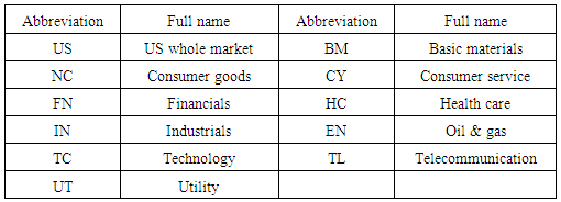
Stock market closely relates to economic conditions. Obviously, stock market flourishes during a booming period and withers during a recession. Because of various characteristics, however, sectoral stock markets may have different processes when co-moving with the economic conditions. In this section we verify this point by analyzing the relationships between sectoral stock returns and the business cycle. Dow Jones Sectoral Indexes system divides the whole stock market into 10 sectors. Table 1 lists the full name and abbreviation of the sectors, including US whole market.Table 1. Basic Sectors and their Abbreviations
 |
| |
|
We follow the abbreviations and use them in the rest of this paper. We also include the whole US market stock index to compare the difference between aggregated and disaggregated market levels.Figure 1 illustrates the relationship between GDP growth rate, representing the business cycle, and sectoral stock returns1. Each panel of this figure draws one sectoral stock returns, which is indicated by a solid red line, together with GDP growth rate, which is indicated by a dashed blue line. In the figure we can see that GDP growth rate fluctuate moderately around zero, with an apparent drop in 2008. While, the stock returns of each sector fluctuates vigorously around GDP growth rate and presents sharp decreases in 2008, according to the recession of US economy in that year. The vertical axis of each panel ranging from -60% to 30% indicates the value of sectoral stock returns and GDP growth rate. Consistent measurement of the vertical axes is very helpful to show the differences among sectoral stock returns. For instance, sector US, NC, and HC are less volatile than others; 2008 recession has strong effects on US, BM, FN, IN, EN, and TC; and the business cycle has opposite effects on sectoral stock returns at some time.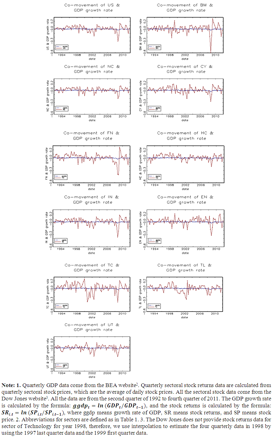 | Figure 1. Co-movement of sectoral stock returns and GDP growth rate, quarterly data |
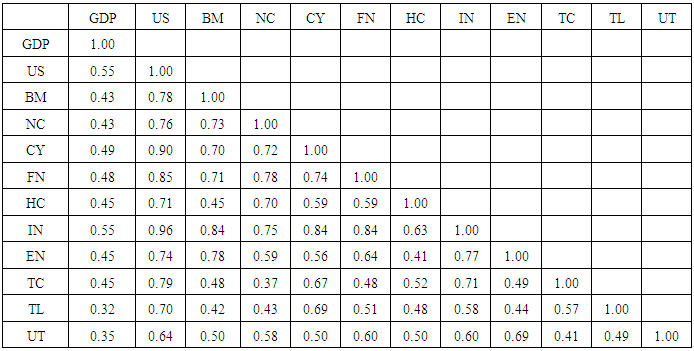
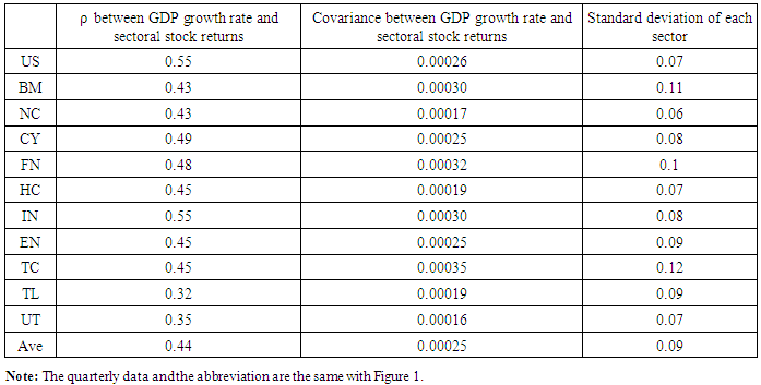
Though GDP growth rate fluctuates moderately but sectoral stock returns fluctuate vigorously, co-movements between them are easy to observe. Table 2 shows the correlation coefficients between each sector and GDP growth rate. The US whole market has the largest correlation coefficient, which is 55 percent. IN also has a high correlation coefficient over 50 percent. There are 7 sectors whose correlation coefficients are higher than 40 percent. The lowest coefficients occur in TL and UT but they still exceed 30 percent. In consequence, we can confirm that, based on quarterly data, all sectors have close relationships with the business cycle. One problem of the constant correlation coefficient is that the largest correlation coefficient occurs on US whole market. Since the US whole market stock index is an average of the sectors, its returns should reflect the average level of them. But in Table 1 the correlation coefficient between US whole market and GDP growth rate is the highest, rather than an average. The reason of this result simply lies in the calculation of the correlation coefficient.In Table 2, we list the covariance between GDP growth rate and the sectors. The average of covariance of all sectors is 0.00025, which is very close to the covariance of the US whole market, 0.00026. The covariance reveals that the whole market index reflects the average level without any ambiguity. However, the comparatively low standard deviation of the whole market boosts its correlation coefficient. The standard deviation of the US whole market is 0.07 which is lower than the average level, 0.09. Three sectors, NC, HC and UT, have smaller standard deviations than the US whole market, but they also have smaller covariances. Other sectors all have larger standard deviations, while their covariances are either smaller than US whole market or not large enough to generate a higher correlation coefficient. The covariances and the correlation coefficients together reveal that the US whole market reflects the average level of the sectors and it also has the closet connection with the business cycle.Table 2. Constant correlation coefficients (ρ) between sectoral stock returns and GDP growth rate
 |
| |
|
Table 3. Correlation (ρ) and covariance between GDP growth rate and each sector
 |
| |
|
Another problem of the constant correlation coefficient is that it reflects a relationship for a long time. Because both GDP growth rate and sectoral stock returns change over time, we need to know the time-varying pattern of the correlations between them. The time-varying correlations are useful in that investors can form investment strategies by diversifying their choices in short time. The DCC-GARCH model can help us find the dynamic correlation coefficients.
3. Dynamic Conditional Correlation Coefficient
3.1. The DCC-GARCH Model
Engle (2002) provides a multivariate GARCH model to calculate the time-varying correlation coefficients between two time series. This model is developed from constant conditional correlation model established by Bollerslev (1990). If each of two random variables follows a univariate GARCH process, then their conditional covariance can be described by their conditional variances times a correlation coefficient:  . The DCC-GARCH model enables correlation coefficient
  to change over time:
  .Preliminary analysis for ACF of sectoral stock returns indicates that their autoregressive order is one:
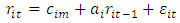 | (1) |
The subscript i indicates different sectors, which are US, BM, NC, CY, FN, HC, IN, EN, TC, TL, UT, and the subscript m indicates that the parameter is used for mean equation. GDP growth rate is also an AR (1) process: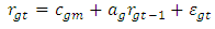 | (2) |
The subscript m has the same meaning and the subscript g indicates GDP growth rate. Residuals of sectoral stock returns and GDP growth rate are assumed to follow GARCH (1,1) processes, and conditional covariance of each sector and GDP growth rate is described by the DCC-GARCH model: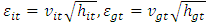 | (3) |
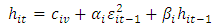 | (4) |
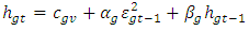 | (5) |
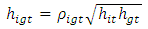 | (6) |
Where  and
and  follow i.i.d. standard normal distributions and
  and
and  are conditional variance of
  and
and  . We can find the conditional covariance between
  and
and  given that these two disturbances are correlated. The time-varying correlation coefficients
  are generated from
 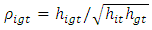 . The problem arises from finding the conditional covariance
  . Following Engle (2002), we use a smoother to estimate it:
 | (7) |
 is the estimate of
  in equation (3), such that
 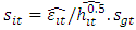 is the estimate of
  in equation (3) and is defined by the same way, such that
 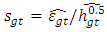 .
.  is the unconditional correlation between
  and
and  . Confining non-negative
  and
and  and
and  assures that the correlations matrix are positive definite and converge to unconditional correlation matrix. Then, the DCCs can be calculated as:
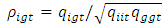 | (8) |
3.2. Estimation of the Parameters
As in Engle (2002), we can use two step estimation to find the parameters in our models. The log-likelihood function of a bivariate GARCH model can be written as: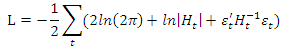 Where
Where  is a vector of the residuals such that
 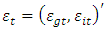 , and
, and  is the conditional covariance matrix of
  . Decomposing
  to a diagonal matrix
  and a symmetric matrix
  allows the log-likelihood function to be estimated by two steps. The conditional covariance matrix
  can be written as
  where
where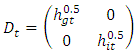 is a diagonal matrix with square root of conditional variances on its diagonal and zeroes otherwise, and
 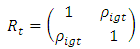 is the symmetric correlation matrix such that
  . Then the third part of the log-likelihood function can be written as
  where
where  is a vector of the standardized residuals such that
  . Therefore, we can write the log-likelihood function as:
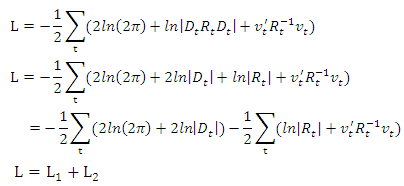 Using
Using  and
and  to represent the two parts of above equation, we find that
  is a function of parameter
  which only contains parameters of the mean and variance equations of GDP growth rate and sectoral stock returns.
  is a function of
  and
and  where
where  only contains parameters of the correlation coefficient equations. Since
  does not depend on
  , we can estimate
  first and then estimate
  . Adding
  into
into  makes
makes  the sum of two univariate GARCH likelihoods
 and subtracting
  from
from  keeps
keeps  unchanged
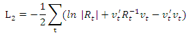 The first step is to estimate
  . Since GDP growth rate and sectoral stock returns do not depend on each other,
  can be estimated as two separate univariate GARCH models. A little more deduction for
  gives us
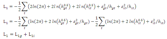 Thus, we break the bivariate log-likelihood function into two parts: a univariate log-likelihood function of the GDP growth rate and a univariate log-likelihood function of sectoral stock returns. Specifically,
  is a function of
  , where
 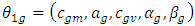 ;
;  is a function of
  , where
 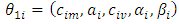 . Because
  does not depend on
  and
and  does not depend on
  , we can estimate
  and
and  as two univariate GARCH process to obtain
  and
and  . The second step is to estimate
  .
.  is a function of
  and
and  where
where  and
and  . Smoother equation (7) and results from
  enable us to estimate
  and derive the smoothers
  by maximizing
  . Then, placing the smoothers
  into equation (8) we can find time-varying correlation coefficients
  .
.
3.3. Empirical Results
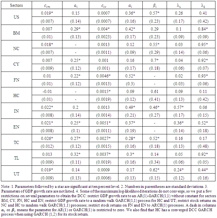
The first column in Table 4 contains estimated values of the constant term  in equation (1). Six of them are significant including US whole market. Parameters for AR(1) terms are in the second column. A dash for NC and HC indicates their AR(1) parameters are restricted to zero in searching for a converged maximum log-likelihood. For the rest sectors, AR(1) parameters are positive and have approximate magnitudes. Columns three to five are parameters for the variance equation. Most of the ARCH(1) and GARCH(1) parameters are significant. In order to obtain a converged maximum log-likelihood, we restrict GARCH(1) parameters for FN and EN to zeros. For some sectors, like NC, the ARCH(1) parameter is small and the GARCH(1) parameter is large. Thus, for these sectors, a shock from last period has a small effect on current volatility but this effect will last for a long time. On the other hand, for some other sectors, like BM, the ARCH(1) parameter is large and the GARCH(1) parameter is small. Thus, for these sectors, a shock from last period has a strong effect on current volatility, but this effect will decay fastly.
Table 4. Estimated parameters of DCC-GARCH model between GDP growth rate and each sector
 |
| |
|
Last two columns are estimates of DCC parameters  and
and  in equation (7). These two parameters should be positive and their sum should be in unit circle to ensure the conditional covariance converging to its long run unconditional level. These two parameters enable sectoral stock returns to accumulate previous shocks and dynamic effects and make the conditional covariance fluctuate along the horizon. The closer the sum of the parameters to unity and the larger the parameter
  , the greater the conditional covariance persists. The closer the sum to zero, the greater the conditional covariance converges to its long run value-the unconditional covariance. The larger the parameter
  , the greater the conditional covariance fluctuates. In our results, the sum of
  and
and  is close to one for BM, NC, CY, FN and TL. These sectors also have a large parameter
  . Therefore, these sectors will have more persistent conditional covariance. The sum of these two parameters is only 0.2 for the sector HC, so the conditional covariance of HC will be closer to its unconditional covariance than other sectors. US, IN, EN and UT have a large parameter
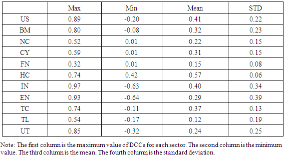
  and their conditional covariances are more volatile than other sectors.In Figure 2, we plot the estimated DCC for each sector in 11 panels along with their constant correlation coefficients. In each panel, a horizontal line is also drawn to indicate the zero value of correlation coefficient. There are some common features of each sector’s DCCs. First, it is easy to see that those DCCs fluctuate around their long run unconditional correlation coefficient, and all of them have a tendency to converge to that. Some sectors have more volatile DCCs, like the US whole market, IN, EN and UT, in observing the large estimates of
  . The largest difference between the DCCs and the constant coefficient occurs on IN, when a negative correlation between the economy and stock returns exits. Second, whether volatile or not, there is a trend in each DCC curve such that the dynamic correlation has continued to increase over the past 20 years. This increasing process reveals that connections between the economic conditions and sectoral stock returns become stronger and stronger. Third, though generally sectoral stock returns are positively and increasingly related to economic conditions, some sectors are found negatively moving along with economic conditions. Comparing to the zero correlation line, negative dynamic correlation coefficients appear on US, BM, IN, EN, TC, TL and UT. During the periods when negative coefficients are observed, diversifications within sectors will benefit investors.
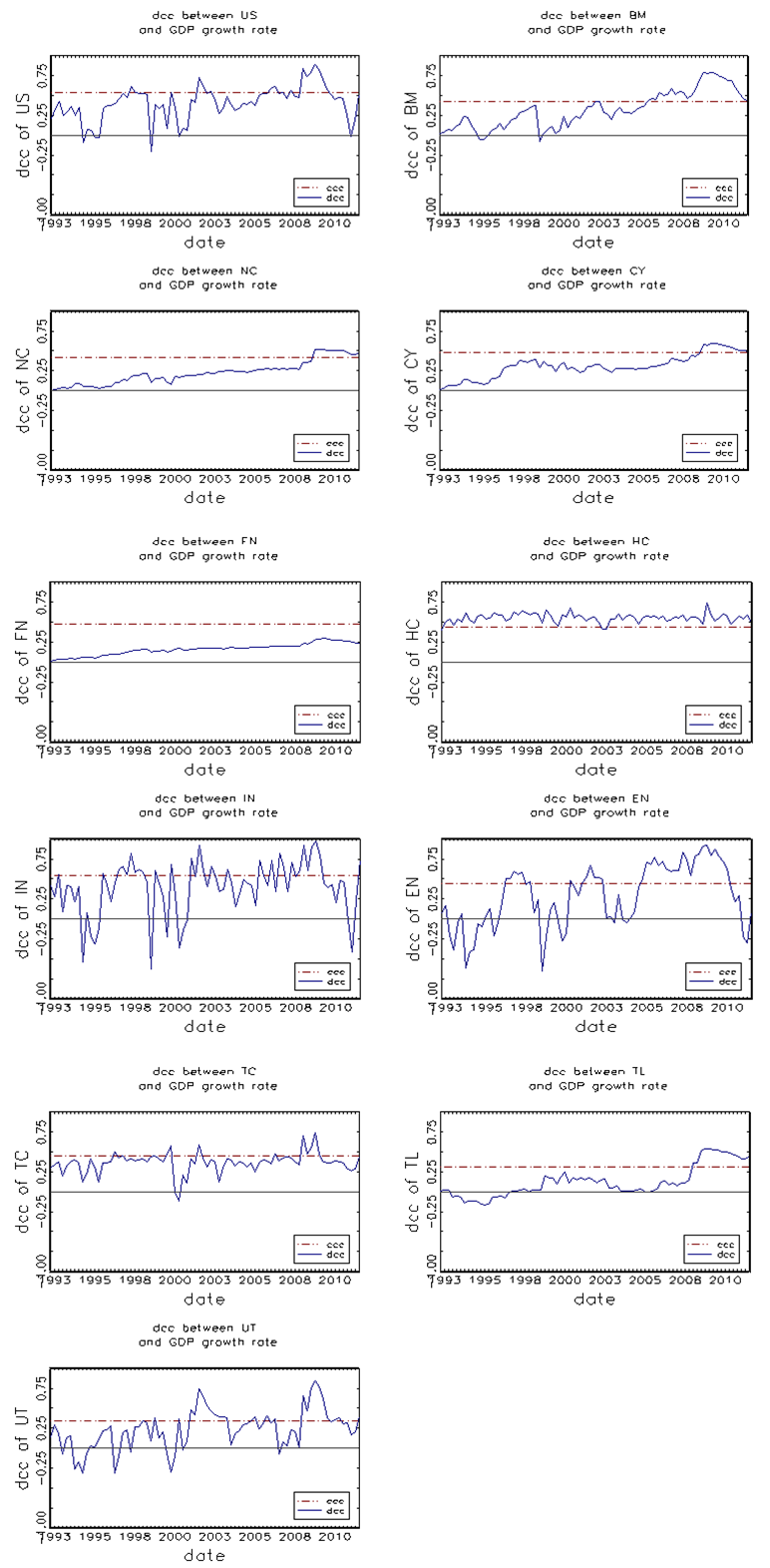 | Figure 2. Dynamic conditional correlation coefficient between GDP growth rate and each sector |
From above analysis, we can confirm that constant correlation is not enough when considering portfolio construction. Dynamic correlation is a more effective method to cope with conditional risk. Some statistics of the estimated DCCs are presented in Table 4.
4. Variation of Sectoral Stock Returns over Business Cycles
4.1. Outlook of Monthly Sectoral Stock Returns over Business Cycles
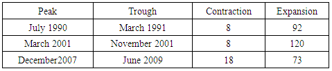
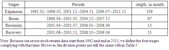
In this section, we investigate the relationship between sectoral stock returns and business cycles directly. We want to add some new evidence to the existing literature, which shows how different sectors move asymmetrically over business cycles. Since the Dow Jones only has recent 20 years sectoral stock indexes data, we focus on the nearest 20 years business cycles. Specifically, the NBER determines three peaks and three troughs in these years, as in Table 54. The lengths of contractions and expansions are also provided in the same table. As denoted by the NBER, a contraction is a period between a peak and the next trough, and an expansion is between a trough and the next peak.Table 5. Statistics of Dynamic conditional correlation for each sector
 |
| |
|
In Figure 3, we plot monthly sectoral stock returns, along with the business cycle information listed in Table 6. Without the data restirction of GDP, which is only available in quarterly frequency, we can use monthly stock returns for all sectors. The shadows in each panel indicate two contractions in recent 20 years. The shadows also divide the rest portions into three parts, which are expansions in business cycles. It is apparent that each series falls under the zero horizon line in the two contractions, especially in the second one. Although there are some negative observations in the expansion periods, most of them are positive. Furthermore, even if being negative, the returns bounce back to positive quickly during expansions. However, the negative values of returns during contraction are more persistent. 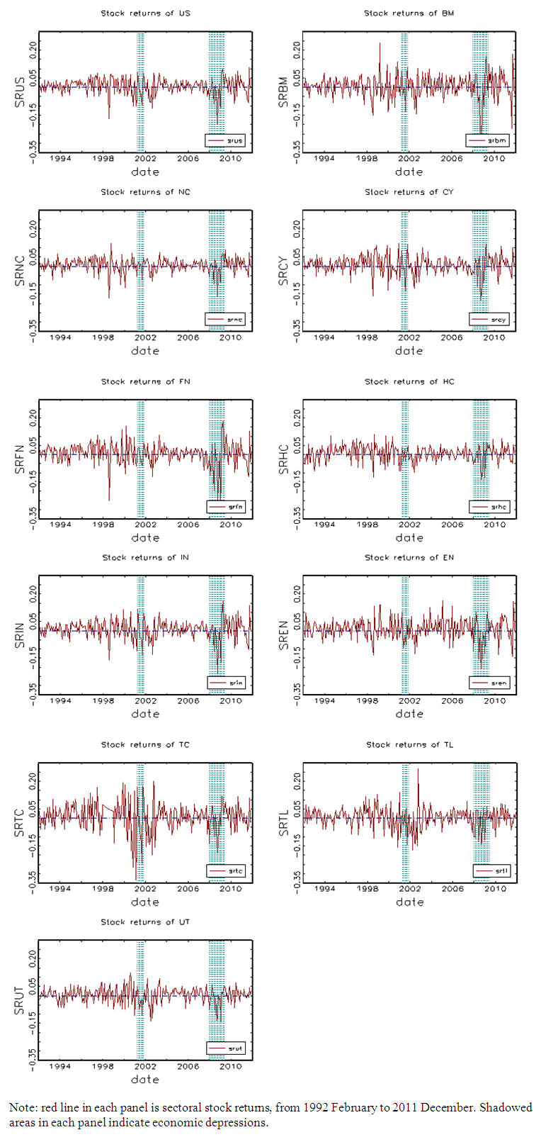 | Figure 3. Sectoral stock returns over business cycles |
Table 6. The NBER Business Cycle information from July 1990 to June 2009
 |
| |
|
Although the sectors share common features, some of them have their own properties. For example, some sectors, like FN and TC, have more variation in the first expansion than in the second one, while, some other sectors do not have much difference in these two periods, like BM and EN. Some sectors have local minimum value in 1999, like the US and FN, but sector BM has a maximum value in the year. Moreover, some sectors, like US and CY, fluctuate more vigorously around the first contraction, but some sectors show the opposite. One interesting sector is Technology, which experiences dramatical volatility from 1999 to 2003. This may arise from the computational innovation during that time. As a consequence, different behaviors of sectors demonstrate the fact that diversification of investment among sectors may be profitable.
4.2. Average Behavior of Sectoral Stock Returns over Business Cycles
Now consider a regression of each sector on business cycles. Expansions and contractions are defined by NBER, as in Table 5. Then, by using the middle point of the time span, we divide an expansion into two stages, which are recovery and prosperity, and divide a contraction into two stages too, which are recession and depression. This method has been used in other papers, like in DeStefano (2004). Table 6 presents the period of time and the lasting length of each stage of business cycles. From the table we can see the four stages jointly form an entire business cycle.We then define four dummy variables corresponding to the four stages as follows: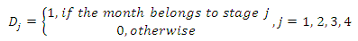 For example,
  is the dummy variable for stage prosperity. Referring to Table 7,
  has value 1 during April 1996 to March 2001 and December 2004 to December 2007, and has value 0 for other periods. Thus, each dummy variable has the same length as the sample period. A regression model is set up to investigate varying performance of sectoral stock returns over business cycles:
 | (1) |
where  to
to  are dummy variables for four stages and
  are parameters related to them. Through the regression on dummy variables, we can separate variation of sectoral stock returns according to different stages.
Table 7. Four stages of business cycles
 |
| |
|
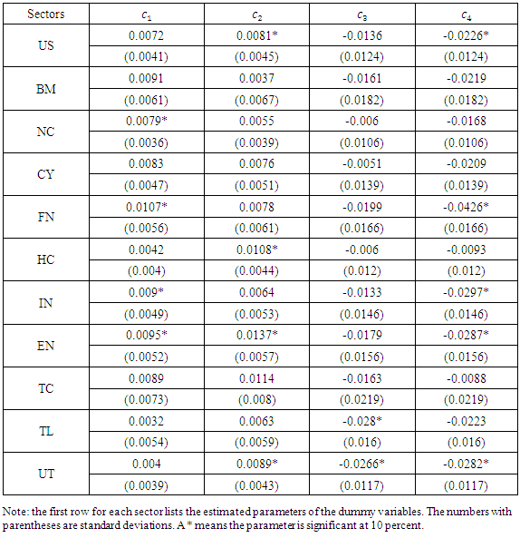
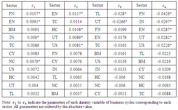
Table 7 presents the regression results on 4 dummy variables of business cycles. Every sector has positive parameters in stage I and stage II, and negative parameters in stage III and stage IV. Therefore, generally speaking, sectoral stock returns and business cycles have positive relationship in expansions and negative relationship in contractions.Specifically, four sectors, NC, FN, IN and EN, have significant estimated parameters in recovery ranging from 0.0079 to 0.0107. Also four sectors, US, HC, EN and UT, have significant estimated parameters in prosperity ranging from 0.0081 to 0.0137. Rest sectors, BM, CY, TC and TL, are not significantly affected by these two stages of business cycles. It is apparent that in prosperities sectoral stock returns have better performance than in recoveries. Only two sectors, TL and UT, have significant parameters in recession which are -0.028 and -0.0266. Five sectors, US, FN, IN, EN and UT, have significant parameters in depression ranging from -0.0266 to -0.0426, in absolute value. It is also clear that depressions have worse effects on sectoral stock returns than recessions. Significant parameters are not observed on BM, NC, CY, HC and TL. One interesting conclusion from these results is that business cycles tend to have stronger effects on sectoral stock returns when approaching to peaks and troughs. From the aspect of the stages of business cycles, stage IV significantly affects five sectors, which is the most compared to other stages. Therefore, exiting in stage IV will guarantee the profit at a higher determinate level. Stage I and II affect four significant sectors, hence entering in this stage may also be profitable. Stage III only significantly affects two sectors, so no clear guideline will be produced in this stage.From the aspect of sectors, EN and UT have the most reliable results. Business cycle effects on them are quite important because all of them have three significant parameters. Therefore, selecting these three sectors in a portfolio will ensure a stable profit. On the other hand, BM, CY and TC have no significant estimated parameters at all. Thus, when using business cycle information to forecast stock returns, investors need to pay close attentions on them. All other sectors have one or two significant stages in business cycles. In Table 8 we re-list the regression results according to parameter values of each dummy variable. All the parameters are sorted by decreasing order of absolute values. Thus, sequences of sectors in columns one and three express the profitability of sectors in recoveries and prosperities; while, sequences of sectors in columns five and seven express the risk of sectors in recessions and depressions. On the basis of this result, in Table 9 we make some suggestions on diversifying portfolios through business cycles. Table 8. Regression results of each sector stock returns on 4 dummy variables of business cycles
 |
| |
|
Table 9. Effects of business cycle on sectoral stock returns: sorted by magnitude of coefficients
 |
| |
|
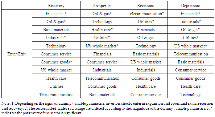
Investors should enter the sectors in recoveries and prosperities following the order of columns two and three, or diversify a portfolio by including more upper sectors. In recessions and depressions, investors should exit the sectors as the order of columns four and five, or change a portfolio by excluding more upper sectors. The stars after sectors indicate that the parameters of the stage dummy variables are significant. These sectors, which will guarantee more reliable results, may be preferred by a risk averse investor.Table 10. Suggestions for portfolio management
 |
| |
|
5. Conclusions
In this paper we use three methods to investigate the relationship between US business cycle and US sectoral stock returns. For the first two methods, we use GDP as a proxy of the business cycle. For the third one, we use dummy variables to represent the business cycle. The conclusion is very clear that the business cycle and sectoral stock returns have close relationships. The constant correlation coefficients between GDP growth rate and sectoral stock returns range from 32% to 55%. The dynamic correlation coefficients between them converge to their constant coefficients and generally have an upward trend. The dynamic correlation coefficients are stable on some sectors but are quite volatile on some other sectors. The largest dynamic coefficient is 97% on IN and the smallest one is -64% on EN. The mean of DCCs of different sectors ranges from 12% in TL in 57% in HL. The empirical results of the second method reveals that constant correlation coefficient has its disadvantage in diversifying portfolios.The time-varying pattern of correlation between macroeconomic variables and sectoral stock returns is also confirmed by some other papers. For example, Caporale, Ali and Spagnolo (2014) investigated DCC between oil price changes and sectoral stock returns in China. Their findings revealed that the average dynamic correlation between oil price changes and sectoral stock returns ranges from 6.1% in UT to 14.9% in EN. Though the correlation they found are smaller than that in this paper, which is because the oil price is only one aspect of the entire macroeconomic environment indicated by GDP, their research is also a strong evidence that dynamic correlation is a better method when diversifying portfolios. Regressions of sectoral stock returns on business cycles show that all sectors have positive parameters in expansions and negative parameters in contractions. Considering a four stage classification, we find that sectors have varying performance through business cycles. Some sectors are influenced intensely by business cycles but some sectors are not affected at all. The multifarious appearances of sectors provide some possibilities to diversify portfolios among sectoral stock markets.
Notes
1. Sometimes we will add the whole US market on the top of sectors and mention them together as “eleven sectors”.2. The website address is: http://www.bea.gov/iTable/iTable.cfm?ReqID=9&step=13. The website address is: http://www.djindexes.com/investable-products/?assetclass=equity&tab=globalindexes.4. The data come from NBER website at: http://www.nber.org/cycles/cyclesmain.html.
References
| [1] | Robert Engle, 2002. Dynamic conditional correlation-A simple class of multivariate GARCH models, Journal of Business and Economic Statistics 20(3), 339-350. |
| [2] | Faruk Balli, Hatice Ozer-Balli, 2011. Sectoral Equity Returns in the Euro Region: Is There Any Room for Reducing Portfolio Risk? Journal of Economics and Business 63, 89-106. |
| [3] | Gregory Koutmos, Anna D. Martin, 2007. Modeling Time Variation and Asymmetry in Foreign Exchange Exposure. Journal of Multinational Financial Management 17, 61-74. |
| [4] | Ilhan Meric, Mitchell Ratner, Gulser Meric, 2008. Co-movements of Sector Index Returns in the World's Major Stock Markets in Bull and Bear Markets: Portfolio Diversification Implications. International Review of Financial Analysis 17, 156-177. |
| [5] | Jean-Pierre Berdot, Daniel Goyeau, Jacques Leonard, 2006. The Dynamics of Portfolio Management: Exchange Rate Effects and Multisector Allocation. International Journal of Business 11, 187-209. |
| [6] | K.C.John Wei, K.Matthew Wong, 1992. Tests of Inflation and Industry Portfolio Stock Returns. Journal of Economics and Business 44, 77-94. |
| [7] | Keran Song, Prasad V. Bidarkota, 2015. Asymmetric Business Cycle Effects on US Sectoral Stock Returns. International Journal of Economics & Management Sciences 4:289. doi: 10.4172/2162-6359.1000289. |
| [8] | Michael DeStefano, 2004. Stock Returns and the Business Cycle. The Financial Review 39, 527-547. |
| [9] | Michel Fouquin, Khalid Sekkat, J. Malek Mansour, Nanno Mulder, Laurence Nayman, 2001. Sector Sensitivity to Exchange Rate Fluctuations. Working papers, CEPII research center. |
| [10] | Mohamed El Hedi Arouri, 2011. Does Crude Oil Move Stock Markets in Europe? A Sector Investigation. Economic Modelling 28, 1716-1725. |
| [11] | Mohamed El Hedi Arouri, Duc Khuong Nguyen, 2010. Oil Prices, Stock Markets and Portfolio Investment: Evidence from Sector Analysis in Europe over the Last Decade. Energy Policy 38, 4528-4539. |
| [12] | Mohamed El Hedi Arouri, Jamel Jouini, Duc Khuong Nguyen, 2011. Volatility Spillovers between Oil Prices and Stock Sector Returns: Implications for Portfolio Management. Journal of International Money and Finance, 30(7), 1387-1405. |
| [13] | Mohamed El Hedi Arouri, Jamel Jouini, Duc Khuong Nguyen, 2012. On the Impacts of Oil Price Fluctuations on European Equity Markets: Volatility Spillover and Hedging Effectiveness. Energy Economics 34, 611-617. |
| [14] | Mohan Nandha, Robert Faff, 2008. Does Oil Move Equity Prices? A Global View. Energy Economics 30, 986-997. |
| [15] | Mun Soo Choi, Daniel Zeghal, 2002. Exchange Rate Exposure and the Value of the Firms. Discussion Paper, University of Ottawa, January. |
| [16] | Tim Bollerslev, 1990. Modelling the coherence in short-run nominal exchange rates: A multivariate generalized ARCH model. The Review of Economics and Statistics 72(3), 498–505. |
| [17] | Guglielmo Maria Caporale, Faek Menla Ali, Nicola Spagnolo. 2014. Oil price uncertainty and sectoral stock returns in China: A time-varying approach. China Economic Review 9, 11-22. |

 Abstract
 Reference
 Full-Text PDF
 Full-text HTML