1. Introduction

Financial distress prediction could be considered as a crucial topic, because it enables investors (shareholders and lenders) to avoid or reduce costs associated with corporate failure. It also helps other stakeholders (i.e. managers, public or private administrations, suppliers and corporate syndicates) to take appropriate measures based on corporate financial risk (default or bankruptcy risk).

Several definitions of the financial distress have been suggested through the literature. For instance, some authors defined it as a liquidity (or cash flow) problem which may lead to bankruptcy as a final state (Aydın, Başar & Coşkun, 2009: 243-256). Whereas, other authors defined distressed companies as those which display a relative weak financial performance in their respective sector (Akıncı & Erdoğan, 1995: 272).

This work investigates the role of accounting variables (financial ratios) in predicting financial distress. The explanatory power of such variables is examined through generalized linear models (logistic regression models) because it is believed that these variables lack the ability to well predict financial distress over some periods of time. In this view, the study intended to bring evidence that financial ratios are not enough in predicting financial distress since they are commonly used as the only type of predictor variables in several research works. In fact, developing more accurate models are for the sake of business stakeholders as mentioned above.

Furthermore, the study examines relationships between all predictor variables and also between these variables and the likelihood (probability) of financial distress. All predictor variables in the models are expected to be negatively related with the probability of financial distress. Aside this, differences between groups (distressed and non-distressed companies) are tested for each financial ratio, expecting significant differences between groups for all financial ratios.

The financial distress modelling considered in this work includes 6 major steps¹. The first step consists of selecting a sample from a given population aimed in the study. The second and the third steps focus respectively on the selection of classification criterions and on a test of differences between the resulting groups. Predictor variables, the statistical (or mathematical) technique for models, and time lags are selected in the fourth step, and models are developed in the fifth step. The last step is for the application of the resulting models and an investigation of their predictive accuracy.

The rest of this paper is organized around four sections. The first one focuses on theories and empirical works linked to financial distress. The second one deals with methodology; especially each step of the financial distress modelling introduced above. Research findings are provided and discussed in the last but one section. Finally, conclusions are drawn in the last section.

2. Literature Review

This section includes theories used to make assumptions in some steps of the financial distress modelling in this work along with a review of some empirical works in the area of financial distress.

2.1. Theoretical Basis

The corporate and financial theories used in this work are as follows:

“Theories of Capital Structure”: They focus on the effects of capital structure (equity and debts) on cost of capital, profitability, and market value. Several approaches were formulated. The approaches suggesting no effect of capital structure decisions on profitability and market value are the Net Operating Approach and the MM’s first theorem. Approaches suggesting otherwise are the Net Income Approach, the Traditional Approach, and the MM’s second theorem. In actual fact, the MM’s second theorem is said to be more valid nowadays because it accounts for tax savings, bankruptcy costs, and agency costs (Ercan & Ban, 2008: 228-236; Doğukanlı, 2015: 143-144).

“The Optimal Contracting View”: This approach suggests that the appointment of executives (top managers) result from an arm’s-length relationship between them and directors or shareholders. Therefore, such relationship might be seen as a powerful source of motivation resulting in lower agency costs (Bebchuk & Weisbach, 2009).

“The Market Psychology”: This approach suggests that investors do not always behave as rational agents because of prejudgments, greed, fear, and other factors affecting the decision process (Korkmaz & Ceylan, 2010: 605; Nofsinger, 2014: 2-5).

Based on the theories given above, assumptions have been formulated to classify companies within the sample into distressed and non-distressed ones and also to provide explanations for some findings.

2.2. Empirical Studies

Main research works conducted in area of financial distress are those of Beaver (1966, 1968), Altman (1968), Meyer and Pifer (1970), Deakin (1972), Sinkey (1979), Ohlson (1980), and Taffler (1983).

Beaver (1968) developed univariate models (using financial ratios especially profitability ratios) predicting financial distress based on 79 distressed and 79 non-distressed firms; as a result, a liquidity ratio (liquid assets/Total debts) was found to be the variable with the highest explanatory power (Altaş & Giray, 2005: 15; Kurtaran, 2010: 131; Salehi & Abedini, 2009: 399-401).

Another work conducted by the same author (Beaver, 1968) considered changes in stock prices as a control variable and the findings showed that common stock returns accurately predict the likelihood of financial distress up to two years in advance (Salehi & Abedini, 2009: 399-400; Tükenmez, Demireli & Akkaya, 2012: 198).

However, Altman (1968) developed a multivariate model using 22 financial ratios and a paired sample of bankrupt and ongoing firms; the resulting Z-score models (based on discriminant analysis) included five financial ratios with a predictive power up to two years prior to bankruptcy, and the overall correct classification rate of each model (t-1 and t-2) were respectively 95% and 72% (Salehi & Abedini, 2009: 402; Terzi, 2011: 4).

Meyer & Pifer (1970) developed a bank’s bankruptcy prediction model using a paired sample (39 distressed and 39 non-distressed banks); the resulting linear model’s overall correct classification rate was 80% (Kurtaran, 2010: 131).

Deakin (1972) compared the models developed by Beaver (1966, 1968) and Altman (1968) and found that, despite the fact that Beaver’s models are univariate, they have the highest predictive accuracy of the financial distress (Kurtaran, 2010: 131).

Sinkey (1979) developed financial distress prediction models using two proxies for accounting information and an unpaired sample of distressed (90 banks) and non-distressed (20 banks); the findings showed that the models’ overall correct classification rates decrease with time especially from 80% at t-1 to 50% at t-6 (Kurtaran, 2010: 132; Salehi & Abedini, 2009: 401).

Petteway & Sinkey (1980) added market-based variables to improve the previous work conducted by Sinkey (1979), and market-based variables were expected to detect the likelihood of financial distress earlier than accounting variables (Salehi & Abedini, 2009: 401).

Ohlson (1980), for the first time, applied logistic regression to predict financial distress and bankruptcy; this technique was applied in order to solve problems inherent in the discriminant analysis (i.e. the assumption of normality in the predictor variables’ distributions); using financial ratios as predictors, the results showed that t-1 model had the best predictive accuracy rather than t-2 model.

Taffler (1983) developed a model for predicting financial distress in the UK manufacturing industry using discriminant analysis and only 4 financial ratios were significant i.e. included in the model (Altaş & Giray, 2005: 15; Liou & Smith, 2006: 5-6).

Some of the recent works conducted in this area and based only on financial ratios are as follows:

Low, Nor & Yatim (2001) used logistic regression to develop a model predicting financial distress; 9 financial ratios, the total assets (as a proxy for firms’ size), and the change in net income (NI)² were used as predictor variables; companies within the sample (26 distressed and 42 non-distressed) were classified based on solvency, also a control group of 5 distressed and 5 non-distressed firms was considered; as a result, the model’s overall correct classification rate was 82.4% and 90% respectively in the main sample and the control group.

Altaş & Giray (2005) developed a model to predict financial distress using financial ratios computed based on financial statements of textile companies listed on Istanbul Stock Exchange. The number of variables reduced through factor analysis, and logistic regression was applied; the model’s overall classification rate was 74.2%.

Canbaş, Çabuk, & Kılıç (2005) developed and compared discriminant analysis, logit and probit models at t-1, using 12 financial ratios obtained from 18 distressed and 22 non-distressed banks; according to the results, the discriminant analysis model yielded an overall correct rate of classification of 90% while logit and probit models yielded 87.5% (Kurtaran, 2010: 132).

However, Benli (2005) developed and compared logit (logistic regression) models and artificial neural network models using 12 financial ratios; the findings showed that the second type of model slightly outperformed the logit model (Kurtaran, 2010: 133).

İçerli & Akkaya (2006) developed a model based on discriminant analysis and using 10 financial ratios obtained from companies listed on Istanbul Stock Exchange; Main finding of the study is that financial distress is less likely to occur in companies with skilled executives (Terzi, 2011: 5).

Salehi and Abedini (2009) developed Z-score (discriminant analysis) models using financial ratios obtained from 30 distressed (delisted) and 30 non-distressed firms (listed on Teheran Stock Exchange); the models yielded overall correct classification rates of 95%, 85.50% and 90% respectively at t-1, t-2 and t-3.

Kurtaran (2010) developed and compared discriminant analysis and artificial neural network models; data spanning from 1997 to 2002 was obtained from 18 distressed banks (i.e. acquired by a deposit insurance agency) and 18 non-distressed (ongoing) banks; the overall correct classification rate of the discriminant analysis model was found equal (91.7%) both at t-1 and t-2; concerning the second type of model, at t-1 the correct classification rate in both groups was 100%, while at t-2 it was 100% and 77.8% respectively for the distressed and the non-distressed group.

Boisselier & Dufour (2011) used the backward stepwise logistic regression to develop a financial distress prediction model; a 1-1 design (paired sample) dataset including 450 distressed and 450 non-distressed (according to the Diane Data Base classification) was used, and the resulting model’s overall correct classification rate was 73.36% with type I error and type II error respectively of 14.75% and 38.54%.

Terzi (2011) developed a discriminant analysis model using 19 financial ratios computed from accounting data obtained from companies in the food sector listed on Istanbul Stock Exchange; the findings showed that only 2 financial ratios (return on asset ratio and debts/equity ratio) were significant to enter the model, and the overall correct classification rate was 90.9%.

Finally, Jabeur & Fahmi (2014) developed and compared discriminant analysis and logit models; a sample including 400 distressed and 400 non-distressed small and medium-sized businesses (according to the Diane Database) was considered with data spanning from 2006 to 2008; 33 financial ratios were used as predictor variables, and main findings are as follows: the discriminant analysis yielded models with overall classification rates of 95.98%, 64.48% and 59,2% respectively at t-1, t-2 and t-3; whereas, the logit models’ overall correct classification rates were 98%, 66.5%, and 60.5% respectively for the same time lags.

3. Methodology

This section focuses on the technique used to develop financial distress prediction models, the sample data, classification criterions (first classification), and variables used in this work.

3.1. Model Specification and Predictive Accuracy Measures

In this work, one type of Generalized Linear Models known as logistic regression was used to predict financial distress. This technique is widely used because of its satisfactory results especially when the outcome variable is binary (Dougherty, 2007: 294; Maindonald & Braun, 2007: 246; Caner & Karan, 2012: 13). Also, this technique does not require predictor variables to be normally distributed as it is the case in discriminant analysis. Finally, this technique was found to be more appropriate than linear regression analysis. In actual fact, if linear models were to be applied, the predicted outcome values could lie out of the range 0-1 due to heteroscedasticity (non-constant error variance), and this would introduce serious bias in the results (Dougherty, 2007: 292-293; Boisselier & Dufour, 2011: 7).

The model specification is as follows (Low et al., 2001: 53):

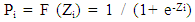
(1)

With;

Pi = (i) subject’s (company) financial distress likelihood (probability).

Exp = Exponential function;

β₀, β₁, β₂, …β_n = Regression coefficients;

X₁, X₂, X₃, …X_n = Predictor Variables;

In actual fact, the model has the aspect of a linear model with an outcome variable referred as Z as showed below (Dougherty, 2007: 293-294):

(2)

Here, the outcome variable could be coded as 1 for subjects with the characteristic of interest (i.e. financially distressed) and as 0 otherwise. Therefore, the outcome variable has to be subjected to transformation (i.e. logarithmic transformation) as showed below:

(3)

Here P_i / (1-P_i) refers to the odds of the event (i.e. financial distress) occurring (Field, Miles & Field, 2012: 319-320); and the likelihood (P-value) of that event occurring could be computed using the Sigmoid function (S) given below (Yıldız, 2009: 59):

(4)

Predictor variables in logistic regression models could be obtained through the maximum likelihood estimation, and the significance level of their coefficients could be tested using the Wald test (Z-statistics) (Field et al., 2012: 313-319; Boisselier & Dufour, 2011: 8). Thus, predictors with coefficients whose Z-values are below a given threshold (e.g. α=0.05) are significant to predict the likelihood of financial distress. The model’s overall significance is tested using the chi-square test and a given threshold; and R-statistics (e.g. Hosmer and Lemeshow R², Cox and Snell's R², Nagelkerke's R²) can be computed to assess goodness-of fit of the model. The relationship between each predictor variable and the likelihood of the event occurring (P_i) can be detected using the odds ratios of the predictor variables’ coefficients (Exp[β_i]) or the confidence interval of each coefficient (Exp[confidence interval]). The relationship between a predictor variable and P_i is negative (resulting in lowering the likelihood of financial distress) when Exp [β_i] or values lying within the confidence interval are below 1; and positive otherwise (Altaş & Giray, 2005: 24; Field et al., 2012: 319-320).

The models’ predictive accuracy could be assessed through classification tables. Such tables cross the observed classification (based on criterions) and the model’s classification, and enable to compute the model’s overall accurate rate of classification, the accurate classification rate in each group (sensitivity and specificity), and type I and type II errors. Nonetheless, classification tables could be misleading because only one threshold (α=0.5) is considered³. As a remedy, Receiver Operating Characteristics (ROC) curves and related Area Under the Curve (AUC) are suggested for use (Hosmer & Lemeshow, 2000: 156-160).

Substantially, the ROC curve accounts for all the possible thresholds by plotting sensitivity on the y-axis and 1-specificity on the x-axis. The graphic is designed to have a diagonal line, and models with a ROC curve as far as possible from the diagonal line are more accurate to detect true positives (i.e. true distressed) and true negatives (i.e. false distressed) which is of help to reduce type II error (Tinoco & Wilson, 2013: 408). False distressed are companies with a high potential of recovery.

In this work, all these procedures were run automatically using the R statistical program and some related add-on packages. Furthermore, stepwise procedures (backward and forward) were applied to select the predictor variables in the models.

3.2. Sample Data

In this paper, the accuracy of financial ratios in predicting financial distress in the Turkish manufacturing industry is to be assessed. The selected sample data only included manufacturing companies listed on Istanbul Stock Exchange. When data was collected, the sample included 194 manufacturing companies⁴. However, some companies were dropped from the sample because of missing data. In actual fact, some companies had data unavailable for 5 consecutive years (2009-2013), and since the first classification was made based on 5 years data, such companies were dropped, bringing the sample size to 133 companies.

As reported in the next sub-section, the first classification resulted in 58 distressed and 75 non-distressed companies. Since 1-1 designs were considered, the final sample data used to develop the models had to include an equal number of distressed and non-distressed companies. Therefore, among 75 non-distressed companies, only 58 companies were picked to match the 58 distressed companies up. The manufacturing industry encompasses sub-sectors (e.g. food, textile, automotive sector), and since some financial ratios (e.g. asset management ratios) does not enable comparison between companies operating in different sub-sectors, each company was matched with a another one operating in the same sub-sector using the NACE 2 classification published by the Turkish central bank⁵. However, some sub-sectors included more distressed companies. Such companies were matched with companies operating in similar sub-sectors.

Three models were developed especially at t-1, t-2 and one based on a crossover design. The year of financial distress (t) was considered as the year in which the company faced more problems (considering profitability ratios and other controls such as abnormal returns). This t year differs from a company to another, but lies within the 2009-2013 period. The t year of non-distressed was set equal to that of the matched distressed company.

3.3. Classification Criterions

Companies within the sample data were classified as distressed or non-distressed according to their 5-years (2009-2013) financial performance. In actual fact, this is related to the definition of financial distress admitted in this work i.e. financially distressed companies are those which display a lower performance relative to the sector’s average performance.

As in Aliouche & Schlentrich (2014), four financial performance measures were selected: two accounting-based variables (the return on assets referred as ROA and the return on equity referred as ROE) and two market-based variables (the economic value added referred as EVA and the market value added referred as MVA⁶). Companies with a 5-years mean ROA or ROE below the 5-years overall mean of the sector were classified as distressed.

Here, Z standardization was applied to easily detect values above and below the sector’s 5-years mean; subjects with negative Z values are those who performed below the mean and those with positive Z values performed above the mean. The Z value is as follows (Anderson, Sweeney & Williams, 2010: 125):

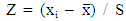(5)

With x_i the observation, the distribution’s mean, and S the standard deviation of the distribution.

In order to avoid serious bias in the classification, the overall ROA mean and ROE mean were computed after applying winsorization at 90% on the distribution of these variables. This technique consists of reducing the influence of outliers on the mean by setting values above the 95^th percentile equal to this percentile, and values below the 5^th percentile equal to this one. In fact, outliers were detected in the distributions of ROA and ROE 5-years mean through boxplot graphics as showed below (“Figure.1” and “Figure. 2”). Furthermore, companies with EVA and MVA 5-years mean values below 0 (negative values) were classified as distressed.

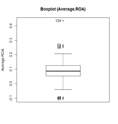Figure 1. Boxplot graphic of the distribution of ROA 5-years mean

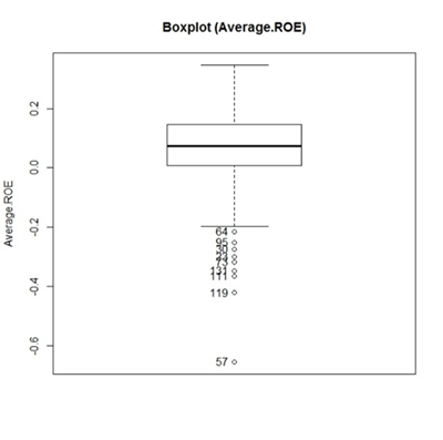Figure 2. Boxplot graphic of the distribution of ROE 5-years mean

Following Tinoco & Wilson (2013), two conditions were also to be met to classify a company as distressed: the first one was based on the earnings before interest, taxes, depreciation, and amortization (EBITDA) i.e. if EBITDA was lower than financing expenses for 2 consecutive years, the company is distressed. The second condition was based on the growth in market value i.e. if the growth in market value was negative for two consecutive years, the company is distressed. For each criterion, status of a company was detected. Thus, the final status of a company was one detected by most of the criterions. However, in some cases divergences between accounting-based and market-based criterions were observed to the extent that only one type of criterion had to be privileged. In these cases, accounting-based criterions were preferred because equity markets could be irrational as explained in the theoretical basis (Market Psychology)⁷. Hence, over a sample size of 133 companies, the classification yielded 58 distressed (44%) and 75 non-distressed companies (56%).

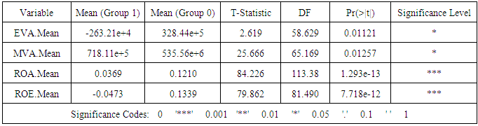
3.4. Classification Assessment

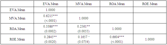
The resulting classification had to be tested before developing financial distress prediction models. In actual fact, a test of equality of means of each group (distressed and non-distressed) was performed according to each variable used to classify companies. The relationship between these variables were also examined through a scatterplot matrix and a correlation matrix (“Figure. 3” and “Table. 1”) in order to assess the overall convergence of these criterions in the classification.

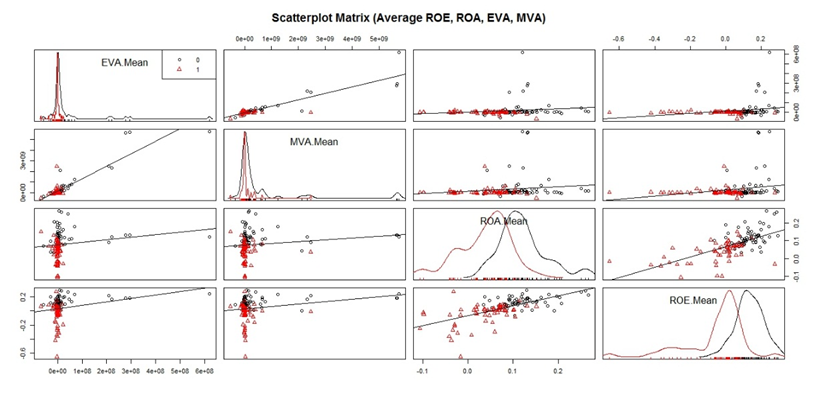Figure 3. Scatterplot Matrix of Variables Used in the First Classification

Table 1. Correlation Matrix of Variables Used in the First Classification8

The given scatterplot matrix shows that all variables are related. This is confirmed by the correlation matrix showing strong relationships between variables especially at 1%-5% significance level, except the relationship between ROE mean and MVA mean which has the lowest significance level (10%). Therefore, all variables used in the classification show convergence between them.

The results of the test of equality of means between both groups and according to variables used in the classification are reported in “Table. 2”. Here, the Welch Two Sample t-test was implemented even though some variables are not normally distributed. In actual fact, this test is more robust than the widely used t-test, and the assumption of variance homogeneity (homoscedasticity) was not assumed. Also, this test yielded the same results (in terms of significance levels) as a non-parametric test known as the Wilcoxon test.

Table 2. Test of Equality of Means between Groups and According to Classification Criterions

“Table. 2” shows that all variables used to classify companies were significant at 1%-%5 levels, suggesting that there is a significant difference between the resulting groups (alternative hypothesis is true). This was confirmed by the error bars graphics (“Figure. 4” and “Figure. 5”)⁹ given below.

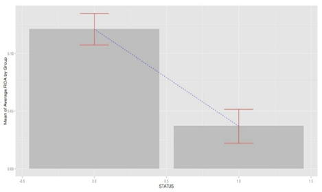Figure 4. Error Bars Graphic for ROA Mean

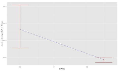Figure 5. Error Bars Graphic for EVA Mean

Since the resulting groups are significantly different, then datasets designed to develop financial distress prediction models could be considered as reliable.

3.5. Variable Selection

The outcome variable to be predicted is the likelihood of financial distress. This variable is qualitative and categorical (being distressed or not), and in order to run analysis, this qualitative variable was coded as 1 and 0 respectively for distressed and non-distressed companies.

As predictor variables, 15 commonly used financial ratios were selected. These ratios were coded according to their respective group as showed in “Appendix. A”, and computed using financial statements¹⁰ published on the public disclosure platform.

Hence, the three datasets (t-1, t-2 and crossover design) included the outcome variable (the financial status observed through the first classification for each company in the final sample data) and 15 financial ratios mentioned above. In order to reduce the bias introduced by outliers, winsorization at 90% was applied to all financial ratios’ distributions as in the previous step.

4. Results

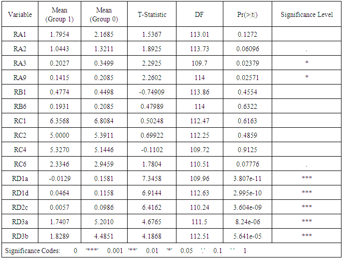
In this section, the relationships between predictor variables, the results of the test of difference between groups (distressed and non-distressed) according to each predictor variable, the resulting models and their predictive accuracy, and the relationships between predictors variables in the models and the likelihood of financial distress (P_i) are reported.

The relationships between each predictor variable used to develop t-1 model (Model I) are reported in Appendix B. According to the table, several financial ratios are related particularly those in the same group of ratios.

Also, partial correlations showed strong relationships between these predictor variables¹¹. This suggests a multicollinearity problem (Gujarati, 2006: 371-376) in the sample data which may result in a few number of variables entering the final models. For t-2 and crossover designs models, the correlation matrix are similar.

For Model I, the results of the test of equality of means between groups and according to each variable are reported in the table below (“Table. 3”)¹².

Table 3. Test of Equality of Means between Groups and According to Predictors in Model I

The test results show that there was not any difference between groups concerning one liquidity ratio (the current ratio RA1), all financial structure ratios, and all asset management ratios (except fixed assets turnover RC6). These results are slightly different for Model II and Model III, but financial structure ratios and assets management ratios remain non-significant even at 10% level, suggesting no significant difference between groups for these ratios.

In actual fact, financial structure ratios were expected to display differences between groups, but according to the finding, it seems like the Net Operating Income Approach and MM’s first theorem are valid. Also, non-significant differences between groups concerning these ratios could be explained through the Optimal Contracting View. In this regard, the executive officers could not take more risks by changing the capital structure regardless of the financial situation. If this assumption is true, then the agency costs would be low in such companies. However, distressed companies have high bankruptcy costs and weak borrowing power, resulting in the capital structure being unchanged.

At t-1, the resulting stepwise logistic regression model (Model I) included 3 predictors as showed below¹³:

(6)

Concerning t-2 stepwise model (Model II), the specified equation is as following:

(7)

Finally, for the stepwise crossover model (Model III), the specified equation is given below:

(8)

The predictive accuracy of the three models are assessed through several measures reported in the table given below (“Table. 4”).

Table 4. Models’ Predictive Accuracy Assessment

The table shows that Model I has the highest R-statistics and overall correct rate of classification, the lowest type II error, BIC and AIC, and the highest AUC¹⁴. Therefore, Model I is the model with the best predictive accuracy. Model III which is for predicting financial distress in the t-1 and t-2 between periods is similar to Model II in terms of predictive accuracy.

Each model’s predictive accuracy was also assessed through a ROC curve as given below¹⁵. Accordingly, the ROC curve of Model I is far from the diagonal line, whereas the ROC curves of Model II and Model III overlap with the diagonal line. Thus, ROC curves confirmed that Model I is the best model.

Here, the ROC curves and AUC show evidence that the classification tables¹⁶ could be misleading. In actual fact, the classification tables of Model II and Model III yielded acceptable overall correct rates of classification (respectively 79.31% and 79.74%), and these rates are close to that of Model I (82.76%). However, according to ROC curves and AUC, Model II and Model III have a low predictive accuracy because they lack ability to detect true distressed and false distressed companies.

Hence, as far as financial distress is concerned, the predictive accuracy of financial ratios decrease with time. The longer the period, the more financial ratios are not reliable in predicting financial distress. However, further research may investigate the role of financial ratios in financial distress prediction for further periods.

The relationships between predictor variables in the best model (Model I) and the related likelihood of financial distress (P_i) are examined in the “Table. 5”.

Table 5. Odds Ratios and Confidence Intervals of Predictor’s Coefficients (Model I)

According to “Table. 5”, two predictor variables (RD1a and RD3a) have odds ratios Exp[βi] and values within the confidence interval below 1. Thus, both variables are negatively related to the likelihood of financial distress. This suggests that, for a given company, as these variables increase the company is less likely to be distressed. However, RD3b has odds ratios Exp[βi] and values within the confidence interval above 1, implying that this variable is positively related to the likelihood of financial distress.

The relationships between predictor variables in Model I and other financial ratios in the t-1 dataset as reported in “Appendix. B” along with the financial statements items which influence these predictor variables have been examined.

Thus, for a given company, if equity capital remains constant, when the net income increases, the return on equity (RD1a) also increases, resulting in lowering the likelihood of financial distress.

Also, if the net income remains constant, RD1a may increase through share buybacks, decreasing the financial distress risk. RD1a was found to be positively related with liquidity ratios. Therefore, it is natural that companies with liquidity problem have higher risk of financial distress. The leverage ratio (RB1) and RD1a were negatively related, but this relationship is not strong (only significant at 10% level). Therefore, changes in capital structure (especially an increase in debts) has somehow an effect on the likelihood of financial distress. Finally, fixed assets turnover ratio (RC6) is also slightly related (at 10% significance level) with RD1a, implying that sales have little effect on the net income¹⁷ and thus on financial distress risk.

The second predictor variable in Model I (interest earned ratio RD3a) is significantly related with all the financial ratios groups except asset management ratios. RD3a is positively related with liquidity and profitability ratios, suggesting that companies with high levels of cash flow have lower financing expenses, and then a lower risk of financial distress. RD3a is significantly related with financial structure ratios (RB1 and RB6). In fact, according to some capital structure theories such as the MM approach (especially the second theorem), as debts increase, the cost of debts (or bankruptcy costs) also increase, resulting in a higher risk of financial distress.

Finally, the relationships between the last predictor variable in Model I (RD3b) and other financial ratios are similar to RD3a. However, RD3b is slightly related with one asset management ratio (RC2).

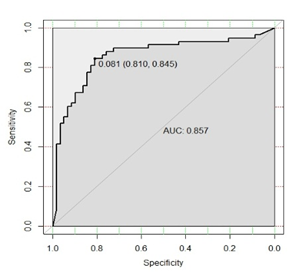Figure 6. ROC Curve (Model I)

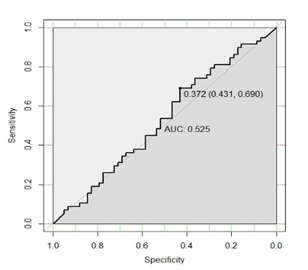Figure 7. ROC Curve (Model II)

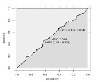Figure 8. ROC Curve (Model III)

5. Conclusions

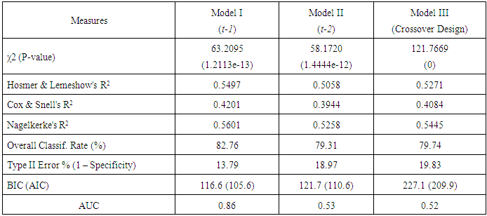
This work’s main purpose was to assess the role of financial ratios in financial distress prediction. In order to do so, models solely based on financial ratios were developed with one year (t-1) and two years (t-2) prior to the event of financial distress. Also, a model based upon a crossover design (t-1 and t-2 data). According to the predictive accuracy of the resulting models, the explanatory power of financial ratios decrease with time, since apart from t-1 model, other models displayed weak performances. This suggests that, in order to get reliable predictions for further periods, other variables (e.g. market variables, macroeconomic variables, corporate governance measures) could be considered. In fact, models with higher predictive accuracy help to better reduce costs associated with corporate failure. Beside this, the findings showed evidence that classification tables (which are the widely used tools to assess the predictive accuracy of financial distress models) could be misleading. To avoid this, ROC curves and AUC could be of help. Finally, it was found that there is no significant difference between distressed and non-distressed companies in terms of financial structure. Accordingly, it was assumed that executive managers do not take more risks by changing the financial structure (especially by increasing debts) regardless of financial situation. And if this assumption is true, then agency costs should be lower in such companies as stated in the Optimal Contracting View. However, the lack of difference in the financial structure of both groups could be due to high bankruptcy costs in distressed companies resulting in lowering their borrowing power.

ACKNOWLEDGEMENTS

This paper is derived from a Master thesis presented in December 2015 at Anadolu University Graduate School of Social Sciences, and titled as follows: “Financial Distress Prediction of Turkish Manufacturing Companies Using Generalized Linear Models”.

The authors would like to thank Özlem Sayılır and Charles Mensah for their helpful advices and comments, along with Yaw F. Ofori-Atta for his help in data collection.

Appendix A. Financial Ratios Used as Predictor Variables

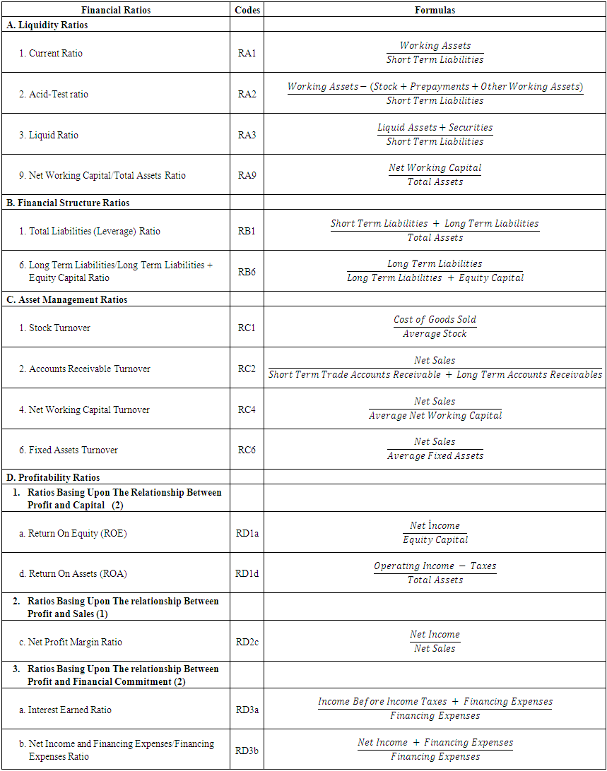Financial Ratios Used as Predictor Variables

Appendix B. Correlation Matrix for Predictor Variables Used in Model I

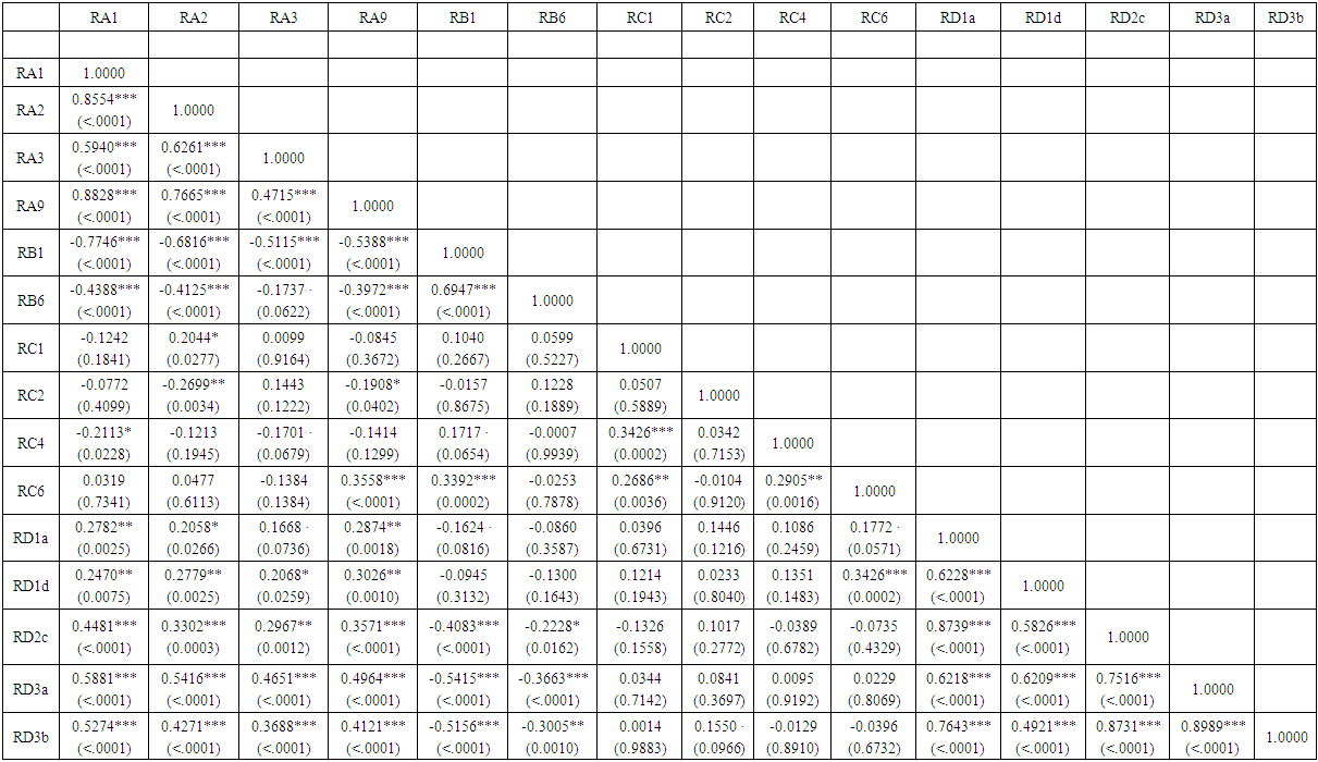Correlation Matrix for Predictor Variables Used in Model I

Notes

1. A pattern of these modelling steps can be provided on request.

2. Computed as in Mckibben (1972) and Ohlson (1980) and as follows: NI = (NI_t – NI_t-1) / (|NI_t| + |NI _t-1|)

3. Subjects with a probability of financial distress (P_i) above or equal 0.5 are more likely to be distressed and those with P_i below the threshold are less likely to be distressed.

4. http://kap.gov.tr/sirketler/islem-goren-sirketler/tumsirketler.aspx (Access date: 23.12.2014).

5. http://www3.tcmb.gov.tr/sektor/2014/Raporlar/NACE_REV2.pdf. (Access date: 28.04.2015).

6. EVA was computed as follows: EVA = Common Equity x (ROE – Cost of Equity); with Cost of Equity = 1/PER as suggested in Chambers (2009: 99-100). MVA was computed as common equity market value minus common equity book value (Aliouche & Schlentrich, 2014: 13).

7. This may also be due to market efficiency.

8. In this work, Spearman correlation coefficients (non-parametric procedure) were preferred to Pearson correlation coefficients (parametric procedure), because, most of variables are not normally distributed as showed in the scatterplot matrix through density plots (Faraway, 2009: 2-5). Values in brackets are the related P-values, and the significance levels are as follows: 0 '***' 0.001 '**' 0.01 '*' 0.05 '.' 0.1 ' ' 1.

9. The graphics show that the error bars do not overlap. Graphics for ROE mean and MVA mean are not reported, but these variables have very similar error bars graphics as ROA mean and EVA mean. Bar charts were added as a layer in the ROA mean’s graphic because this variable is approximately normally distributed.

10. Some financial statements (balance sheets and income statements) were consolidated ones.

11. Partial correlations were obtained through the Holm’s method and could be provided on request.

12. As in the previous section, a more robust t-test (Welch t-test) was implemented. For the other models, the test results can be provided on request.

13. The significance levels for the intercept (1.1392) and the three predictors have been given and are as follows:

0 '***' 0.001 '**' 0.01 '*' 0.05 '.' 0.1 ' ' 1.

14. As reported in Hosmer & Lemeshow (2000: 162); if AUC = 0.5 then the model lacks ability to detect true positive and false negative; if 0.7 ≤ AUC < 0.8 the discrimination is acceptable; if 0.8 ≤ AUC < 0.9 the discrimination is excellent; and if AUC ≥ 0.9 the discrimination is outstanding.

15. The ROC curves are drawn using the “pROC” add-on package in R (Robin, Turck, Hainard, Tiberti, Lisacek, Sanchez & Müller 2011: 12-77).

16. The classification tables can be provided on request.

17. This is probably due to the fact that, for some companies in the sample data, the net income is related to consolidated income statements.