H. G. Dikko1, O. E. Asiribo2, A. Samson1
1Department of Mathematics, Ahmadu Bello University, Zaria, Nigeria
2Department of Statistics, Federal University of Agriculture, Abeokuta, Nigeria
Correspondence to: A. Samson, Department of Mathematics, Ahmadu Bello University, Zaria, Nigeria.
| Email: |  |
Copyright © 2015 Scientific & Academic Publishing. All Rights Reserved.
Abstract
This study models abrupt shift in time series using indicator variable. Seven symmetric and five asymmetric models were considered by incorporating an indicator variable in the variance equation to monitor the changes of some selected Nigerian insurance stocks. The results showed that the daily returns were stationary but not normally distributed and eight out of ten stocks considered for the study showed evidence of ARCH effect. The performance of the different models was evaluated using the RMSE, MAE and MAPE. The model ARCH (1) proved to be the most suitable among the twelve competing volatility models considered. When the regime changes are incorporated into the model, it is found that the highly persistent volatility of the insurance stock return rate is reduced for most of the stocks.
Keywords:
Volatility, Heteroscedasticity, Root Mean Square Error, Indicator variable
Cite this paper: H. G. Dikko, O. E. Asiribo, A. Samson, Modelling Abrupt Shift in Time Series Using Indicator Variable: Evidence of Nigerian Insurance Stock, International Journal of Finance and Accounting , Vol. 4 No. 2, 2015, pp. 119-130. doi: 10.5923/j.ijfa.20150402.02.
1. Introduction
Dummy variables are variables that can take any values. They may be explanatory or outcome variables; however, the focus of this study is explanatory dummy variable construction and usage. Typically, dummy variables are used in the following applications: time series analysis with seasonality or regime switching; analysis of qualitative data, such as survey responses. Some scholars have argued based on statistical analysis of time series that certain phenomena do not correspond to regime shifts, [9]. Outliers, level shifts, and variance changes are common in applied time series analysis. However, their existence is often ignored and their impact is overlooked, for the lack of simple and useful methods to detect and handle those extraordinary events. The problem of detecting level shifts, and variance changes in a univariate time series is considered. Three different types of regime shift (smooth, abrupt and discontinuous) are identified on the basis of different patterns in the relationship between the responses. The smooth regime shifts is represented by a quasi-linear relationship between the response and control variables. The abrupt regime shift exhibits a nonlinear relationship between the response and control variables, and the discontinuous regime shift is characterized by the trajectory of the response variable differing when the forcing variable increases compared to when it decreases see [5].In order to apply the concept to a particular problem, one has to conceptually limit its range of dynamics by fixing analytical categories in time by considering the event and categorically applying it in achieving the significant of the study.In this study we model the abrupt shift in a time series where the variable under study exhibits a nonlinear relationship between the response and control variables using some of the insurance company as a case study, that is, from stable and unstable economic. Therefore our indicator variable will take in the value of 0 for stable and 1 for unstable economy in order to study the abrupt shift in time series since we are considering a time series data to observe these nonlinear relationship in each of the stock with seven symmetric and five asymmetric models incorporating an indicator variable in the variance equation.
2. Literature Review
ARCH and GARCH models, which stand for autoregressive conditional heteroscedasticity and generalized autoregressive conditional heteroscedasticity, have become widespread tools for dealing with heteroscedastic time series. The goal of such models is to provide a volatility measure – like a standard deviation -- that can be used in financial decisions concerning risk analysis, portfolio selection and derivative pricing. Applications of the ARCH/GARCH approach are widespread in situations where volatility of returns is a central issue. Many banks and other financial institutions use the idea of “value at risk” as a way to measure the risks faced by their portfolios. [7] first proposed the autoregressive conditional heteroscedasticity (ARCH) model for modeling the changing variance of a time series; Engle used an ARCH model to study inflation in the United Kingdom. [3] showed that a GARCH model with a small number of terms may be more efficient than an ARCH model with many terms. Empirical studies in recent years have focused on volatility investigation on the pattern of financial assets such as ARCH effect, volatility clustering, and persistence and leverage effect. For example, [23], [18], [24], [21]. The use of dummy variables requires the imposition of additional constraints on the parameters of regression equations to obtain estimates for the model. Among the possible constraints the most useful are (a) to set the constant term of the equation to zero, or (b) to omit one of the dummy variables from the equation. In econometrics time series analysis, dummy variables may be used to indicate the occurrence of wars or major strikes. Dummy variables are used frequently in time series analysis with regime switching, seasonal analysis and qualitative data applications see [5]. Dummy variables are involved in studies for economic forecasting, bio-medical studies, credit scoring, response modelling, etc.[2] used dummy variable to compare the year 2012 internally generated revenue (IGR) and wage bills of the six geopolitical zones in Nigeria by categorizing the geopolitical zones as dummy variables in a regression model to find out if the average internally generated revenue and wage bills of the geopolitical zone are statistically different from each other. From his analysis, he concluded that the northeast and northwest zones are statistically different. [19] used GARCH models with dummies to study the impact of U.S monetary policy on inflation. From the analysis, he concluded that the impact of U.S monetary policy on inflation is negative but not significant on the parameter of the dummy variable the parameter. Stock return volatility represents the variability of stock price changes during a period of time. This phenomenon has attracted growing attention of academia, policy makers and other players in this sector. This is because return is a major measure of risk associated with asset instead of price because if you want an investment that gives 10% of your return you invest on it than in price i.e. it is much better to deal with return than price. Also, high volatility in stocks, bonds and foreign exchange markets usually raise from important public policy issues about stability of financial market and impact of stock volatility on the economy cannot be sub estimated. [17] used volatility to model four Nigerian firms listed on the Nigerian Stock Exchange. [16] also conducted another study which focused on the impact of the 2005 recapitalization of the banking and insurance industry on the stock market. [6] carried out a research on modelling and forecasting daily returns of Nigerian insurance stock using [7] proposed model and [14] to estimate suitable models in, from the study the researcher concluded that the exponential generalized autoregressive conditional heteroscedastic (EGARCH) models is more suitable in modelling stock price returns as it outperforms the other models in goodness of fit and out-of-sample volatility forecasting.
3. Methodology
Data for this study were obtained from daily closing prices of insurance stocks traded on the floor of the Nigerian Stock Exchange (NSE) from 2nd January 2000 to 26th May, 2014. The ten insurance company used for this study are AIICO, GUINEAINS, GUINNESS, LASACO, LAWUNION, NEM, NIGERINS, PRESTIGE, UNIC AND WAPIC.List of Tests and ModelsModels specification 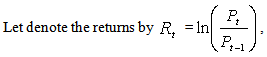 | (1) |
where  and
and  are the present and previous closing prices and
  been the continuously compounded return series because is simply the sum of continuously compounded one-period returns involvedJarque-Bera Test for normalityJarque-Bera is a test statistic for testing whether the series is normally distributed. The test statistic measures the difference of the skewness and kurtosis of the series with those from the normal distribution. The statistic is computed using the expression:
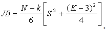 where S is the skewness, K is the kurtosis, and k represents the number of estimated coefficients Under the null hypothesis of a normal distribution, the Jarque-Bera statistic is distributed as a
  with 2 degrees of freedom. Stationary Test (Augmented Dickey-Fuller test)Stationarity of the return series is one of the major assumptions in financial time series modelling. This assumption can be checked using a unit root test. The Augmented Dickey–Fuller test (ADF) is a test for unit root in a time series. Null hypothesis is
  and alternative hypothesis is:
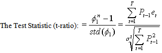 | (2) |
The null hypothesis is rejected if the calculated value of t is greater than t critical value from nonstandard distributions table. Test for ARCH effect (Test for heteroscedasticity)One of the most important issue before consider Heteroskedastic models is examine the residuals for evidence of heteroscedasticity. To test for the presence of heteroscedasticity in residuals of Nigerian insurance stock return series, the Lagrange Multiplier (LM) test for ARCH effects proposed by Engle (1982) is applied. In summary, the test procedure is performed by first obtaining the residuals  from the ordinary least squares regression of the conditional mean equation which might be an autoregressive (AR) process, moving average (MA) process or a combination of AR and MA processes; (ARMA) process using EViews 7 statistical software. For example, in ARMA (1,1) process the conditional mean equation will be as:
 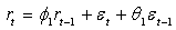 | (3) |
After obtaining the residuals  the next step is regress the squared residual on a constant and its q lags as in the following equation:
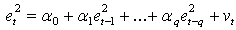 | (4) |
The null hypothesis that there is no ARCH effect up to order q can be formulated as: | (5) |
against the alternative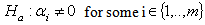 | (6) |
The test statistic for the joint significance of the q-lagged squared residuals is the number of observations times the R-squared  from the regression.
  is tested against
  distribution. This is asymptotically locally most powerful test.Volatility modelsThese models include the symmetric and asymmetric volatility models. The models are ARCH(1), ARCH(2), ARCH(3), GARCH(1, 1), GARCH(2, 1), GARCH(1, 2), GARCH(2, 2) E GARCH (1, 1), EGARCH (1, 2), EGARCH (2, 1), EGARCH (2, 2) and TARCH(1, 1). In each model we incorporated dummies variables.ARCH Models (Autoregressive Conditional Heteroskedastic Model)The ARCH(q) as proposed by Engle is given by
  | (7) |
where  for i=0, 1, 2… q are the parameters of the model.ARCH model with dummy variable
 | (8) |
where  is the dummy variable added to the conditional variance model.GARCH Model (Generalize Autoregressive Conditional Heteroskedastic Model)The GARCH(p,q) as proposed by Nelson is given by
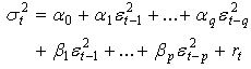 | (9) |
where  and
and  for all i and jGARCH model with dummy variable
 | (10) |
Where  is the dummy variable added to the conditional variance model. TARCH (p,q)Threshold GARCH Model or TARCH (p,q), (Glosten et al.1993) is
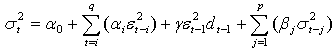 | (11) |
where  if
if  and
and  otherwise. In this model, good news
  and bad news
 have different effects on the conditional variance.TARCH (p, q) with dummy variable
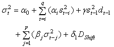 | (12) |
where  is the dummy variable added to the conditional variance model.The E-GARCH (p, q) is given by as proposed in Nelson (1991):
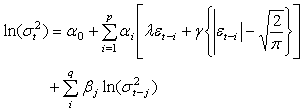 | (13) |
 are the parameters of the model. If p =1 and q =1, the model above reduces to EGARCH (1, 1) given as
 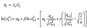 | (14) |
where  are the parameters of the model. EGARCH (p, q) Model with dummy variable is given as
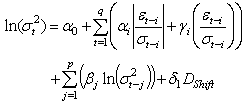 | (15) |
where  is the added dummy variable to the conditional variance model.Goodness of fits certeriaAkaike Information Criteria (AIC) and Schwarz Criteria (SIC) are the most commonly used model selection criteria
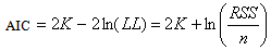 | (16) |
where  is the residual sum of squares.Forecast error statisticsThe forecast error statistics used in this study are the root mean square error (RMSE), mean absolute error (MAE) and the mean absolute percentage error (MAPE). These forecast error statistics are defined by:
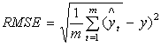 | (17) |
 | (18) |
 | (19) |
where,  with
with  and
and  denoting the number of forecasts, volatility value and the forecast, respectively.The RMSE and MAE depend on the scale of the dependent variable and the differences between volatility value and the forecasted values. The smaller the error statistic is, the better the forecasting ability of that model in consideration of that measure. The MAPE is scale invariant. The satisfactory forecasting model is expected to have MAPE close to 0% which indicate the best forecasting performance to the data.
4. Analysis Result
4.1. Preliminary Result
An initial descriptive statistics analysis of the ten Nigerian Insurance stocks were carried out and the result shown in Table 1. The obtained result as shown in Table 1, showed that the Mean return series for some of the insurance were negative indicating that these insurances incurred loss during the period under study. Despite this loss, two of the Insurances still reported positive return. Also, the result of Jarque-Bera statistic revealed that the return series for all the insurance were not normally distributed as the p-values were less than 1% and 5%.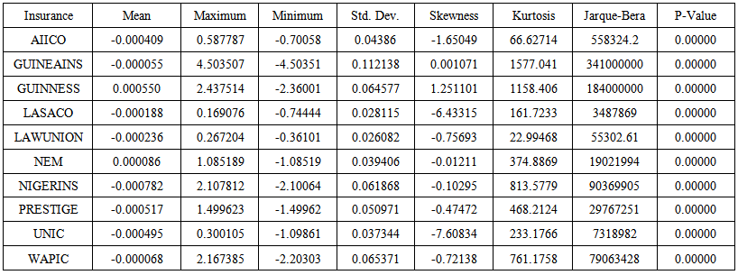 | Table 1. Descriptive Statistics of the return of Nigerian Insurance stocks |
4.2. Analysis of the Main Result
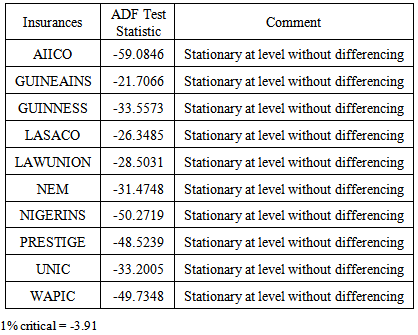
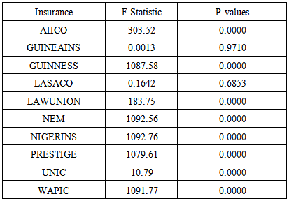
In Table 2 below, the return series were all stationary. Hence, there is no unit root. Therefore, there is no need for differencing. In the Test for ARCH effect, the Lagrange Multiplier (LM) test proposed by Engle (1982) was applied. The F Statistic and the obtained p-values are summarized in Table 3. The results of F Statistic were significant at 1% for eight insurance stock returns while two of the insurance does not exhibit heteroscedasticity. Therefore we cannot run the heteroscedasticity model on them because they do not fulfill the condition of ARCH effect.Table 2. Augmented Dickey-Fuller Test of stationarity test (ADF) of the return series of Nigerian Insurance stocks
 |
| |
|
Table 3. Lagrange Multiplier test of the presence of ARCH effect
 |
| |
|
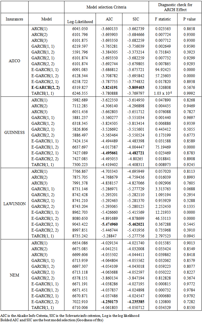
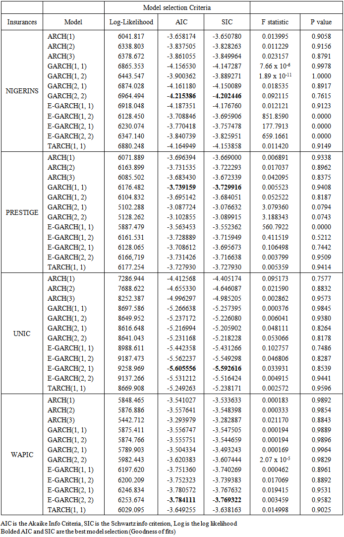
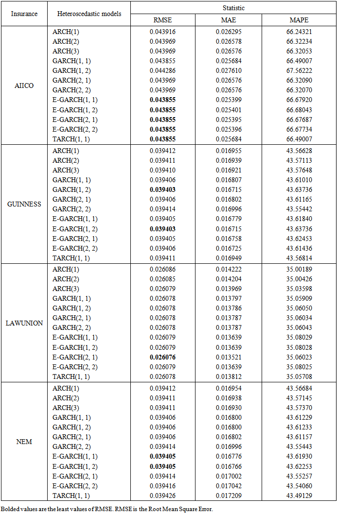
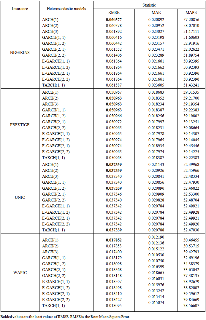
Twelve different heteroscedastic models were fitted by adding a dummy variable to the conditional variance model to test the significance of the hypothesis of the model on each of the model. For AIICO Insurance, all heteroscedastic models fitted had all their parameters significant (p< 0.05) except that some of the model in the abrupt shift showed a positive values with significant level of 0.01.Moreover, NEM, PRESTIGE and UNIC the parameters estimated were significant except the leverage effect of the TARCH (1, 1) model (p>0.05). For PRESTIGE Insurance, the indicator variable is positive throughout the models indicating that the shift was positive. I.e. the global melt down did not affect it. Results are presented in Table 6 and Table 7 with others insurance stocks.Out of the twelve competing models, the selection of the model that could give best prediction was carried out using the Log likelihood (LL), Akaike Info Criteria (AIC) and Schwartz Information Criterion (SIC). Schwartz Information has been considered to be the best of these criteria to as SIC give the heaviest penalties for loss of degrees of freedom (Afees and Ismail, 2012). Hence, it was EGARCH (2, 2) for AIICO, NEM, WAPIC and EGARCH (2, 1) for GUINNESS, LAWUNION, UNIC and TARCH (1, 1) for NIGERINS and PRESTIGE. Results are presented in Table 6 and Table 7.Forecasting performance of these estimated models were investigated using our sample data and statistics like Root Mean Square Error, Mean Absolute Error as well as the Mean Absolute Percentage error were computed. Model with the smallest Mean Square Error was considered to the most suitable for forecasting. Hence, from the results obtained showed that some insurance stocks are having model than one model suitable. Therefore we are going to adopt the Principle of Parsimony – “that the best model is the simplest model that can captures the important features of the data”. Hence EGARCH (1, 1) proved to most suitable for AIICO and NEM, LAWUNION is EGARCH (2, 1), GUINNESS is GARCH (1, 2) while ARCH (1) for NIGERINS, UNIC and WAPIC while ARCH (2) suitable for PRESTIGE. The results are shown in Table 5 and 6.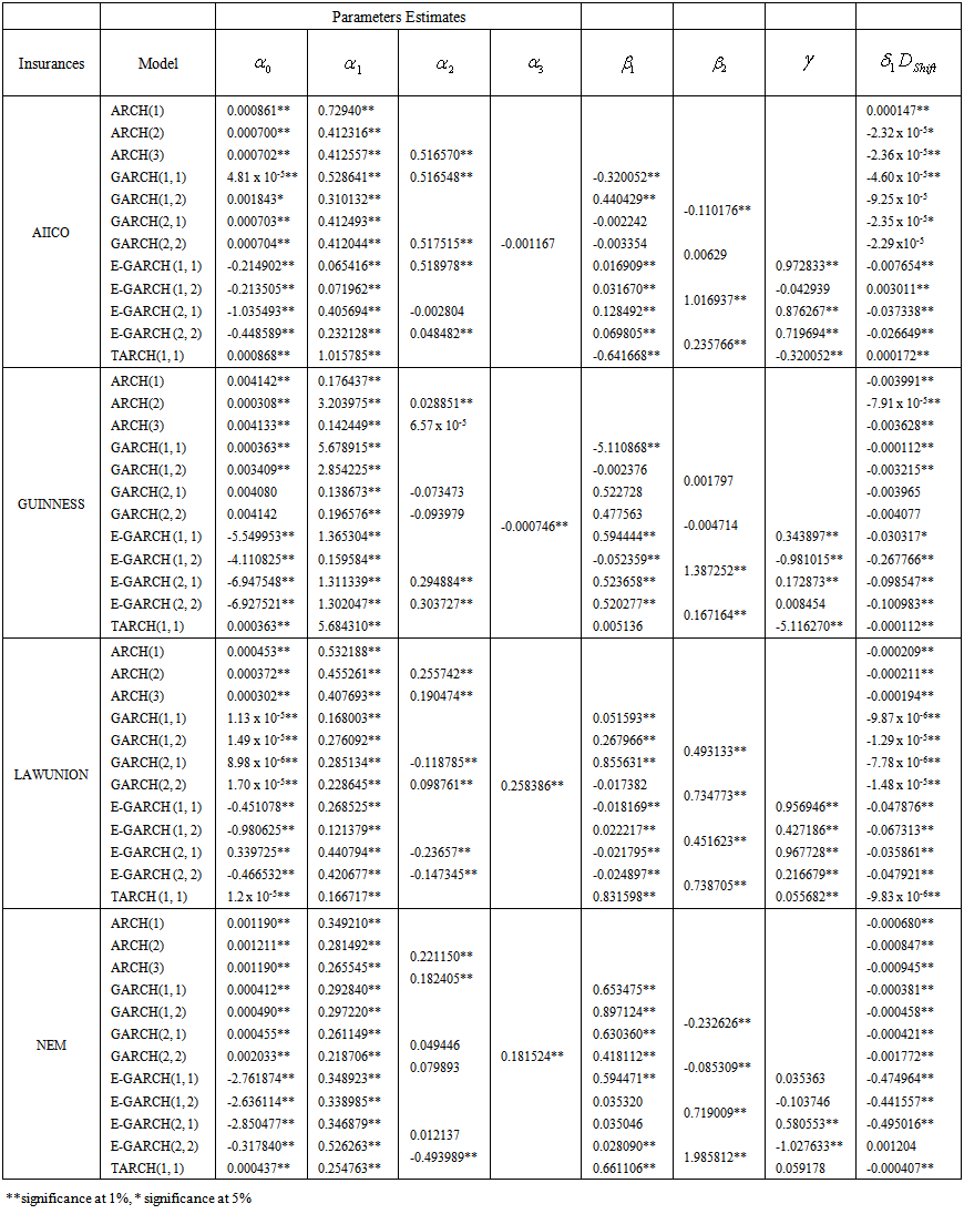 | Table 4. Parameter Estimates of the heteroscedastic models of AIICO, GUINNESS, LAWUNION and NEM |
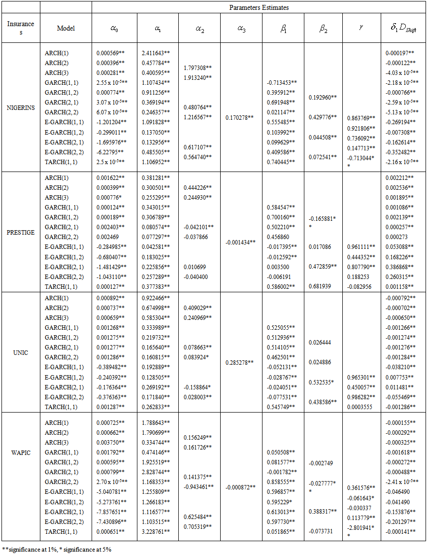 | Table 5. Parameter Estimates of the heteroscedastic models of NIGERINS, PRESTIGE, UNIC and WAPIC |
Table 6. Model Selection criteria (Goodness of fit criteria and diagnostic checking) of AIICO GUINNESS, LAWUNION and NEM
 |
| |
|
Table 7. Model Selection criteria (Goodness of fit criteria and diagnostic checking) of NIGERINS, PRESTIGE, UNIC and WAPIC
 |
| |
|
Table 8. Forecast Performance of estimated model of AIICO, GUINNESS, LAWUNION and NEM
 |
| |
|
Table 9. Forecast Performance of estimated model of NIGERINS, PRESTIGE, UNIC and WAPIC
 |
| |
|
5. Conclusions
This study had examined the daily return volatility of Nigerian Insurance sector stocks. The best model was computed using the AIC and SIC, the bolded models are considered the best fits model to be used in each of the stocks. The forecasting performance of several variants of conditional heteroscedasticity volatility models were evaluated using model evaluation performance measures like the Root Mean Square Error. The post estimation evaluation carried out revealed various conditional heteroscedasticity models to be most suitable for modelling the return pattern of the each insurance. The EGARCH (1, 1) was suitable for AIICO and NEM, LAWUNION is EGARCH (2, 1), GUINNESS is GARCH (1, 2) while ARCH (1) for NIGERINS, UNIC and WAPIC while ARCH (2) suitable for PRESTIGE. But looking at the insurance and by evaluation one can say ARCH (1) was most suitable followed by EARCH (1, 1). This finding is very crucial and informative to investors and intending investors who might want to invest in insurance stocks.
References
| [1] | Ajab A. Alfreedi, Zaidi Isa and Abu Hassan.(2012)"Regime Shift in asymmetric GARCH models assuming heavy-tailed distribution: evidence from GCC stock markets." Journal of Statistical and Econometric Method: 43-76. |
| [2] | Alabi Oluwapelumi.(2014) "Incorporating Dummy variable in Regression Model to Determine the Average Internally Generated Revenue and Wage Bill of the Six Geopolitical Zones in Nigerian.": 23-27. |
| [3] | Bollerslev, Tim. (1986). “Generalized Autoregressive Conditional Heteroscedasticity”. Journal of Econometrics, 31, 307-327. |
| [4] | Brooks, C. (2008). Introductory econometrics for finance. (2nd ed.). Cambridge: Cambridge University Press, (Chapter 8). |
| [5] | Collie, J., et al. (2004) Regime shifts: can ecological theory illuminate the mechanisms? Prog. Oceanogr. 60, 281–302. |
| [6] | Dallah H and Ade I. (2010) "Modelling and Forecasting the Volatility of Daily Returns of Nigerian Insurance stocks." International Business Research, 106-116. |
| [7] | Engle, R. F. (1982). “Autoregressive Conditional Heteroscedasticity with Estimates of the Variances of United Kingdom Inflation”. Econometrica, 50, 987-1007. |
| [8] | Engle, R. F. (2001). “Autoregressive Conditional Heteroscedasticity with Estimates of the Variances of United Kingdom Inflation”. Econometrica, 157-168. |
| [9] | Feng, J.F., et al. (2006) Alternative attractors in marine ecosystems: A comparative analysis of fishing effects. Ecological Modelling 195, 377–384. |
| [10] | Glosten, L. R, Jagannathan, R., &Runkle, D. E. (1993).“On the Relation between the Expected Value and the Volatility of the Nominal Excess Returns on Stocks”. Journal of Finance, 48(5), 1779-1791. |
| [11] | Lawford, Steve. (2004) “Finite-sample quantiles of the Jarque-Bera test. Department of Economics and Finance”, Brunel University, p. 7. |
| [12] | Longmore R, Robinson W. (2004). Modeling and Forecasting Exchange Rate Dynamics: An Application of Asymmetric Volatility Models. Bank. Jamaica, Res. Serv. Dept., WP 2004/03. |
| [13] | Moustafa, A.A (2011). “Modelling and forecasting time varying stock return volatility in the Egyptian stock market”. International Research Journal of Finance and Economics, 78, 1450-2887. |
| [14] | Nelson, D. B. (1991). “Conditional heteroskedasticity in asset returns: A new approach”. Econometrica, 59, 347-370. |
| [15] | Olowe R.A. (2009a) "Stock return colatility and the global financial crisis in an emerging market: The Nigerian Case." International Research Review of Business Research Paper 426-447. |
| [16] | Olowe R.A. (2009b) "The Impact of the announcement of the 2005 capital requirement for insurnace compaines on the Nigerian Stock market." Nigerian Journal of Risk and Insurance, 43-69. |
| [17] | Onwukwe C.E, Bassey B.E and Isaac I.O. (2011) "The Volatility of Nigerian Stock Returns Using GARCH Models.", Journal of Mathematics Research Vol 2, 50-62. |
| [18] | Pesaran B and Robinson G. (1993) "The European Exchange Rate Mechanism and Volatility of the Sterling-deuctmark Exchange Rate.", Economic Journal, Vol 1.1418-1431. |
| [19] | Scott Deacle. (2006) "GARCH models with dummies: A Study of the Impact of U.S Monetary Policy on Inflation." Economic Journalpp28-48. |
| [20] | Sulimon, Z.S (2012). Modelling stock return volatility: Empirical evidence from Saudi Stock Exchange: International Journal of Finance and Economics, 85, 167-179. |
| [21] | Taylor, S. J. (1986). “Forecasting the Volatility of Currency Exchange Rates”. International Journal of Forecasting, 3, 159-170. |
| [22] | Tsay L.S. “Analysis of Financial time series”. Second edition, Hoboken, NJ Wiley, 2005. |
| [23] | Tse Y.K and Tsui A.K. (1997) "Conditional Volatility in Foreign Exchange Rates:Evidence from the malaysian Ringgit and Singopore.", Pacific Basin Finance Journal, 256-345. |
| [24] | Yoon T.A and Lee K.S. (2008) "The Volatility of Future Currency Option Imply Volatility of Exchange Rates." Journal of Social Sceince,Vol 1, 7-9. |
 Abstract
 Reference
 Full-Text PDF
 Full-text HTML