1. Purpose

The purpose of this study is to show that the whole financial system is becoming a Cash-flow system where a continuous adjustment of the variables affecting the discounted present value of the cash-flow stream will show its effect on the value of the company’s stock. Our Financial System would react to the cash-flow and corporation reacts to what investors react and vice versa. All investors operate on time value of money. From here rises a cash flow concept of profit associated with the cash-flow theory of stock valuation.

This theory of stock valuation is based on the assumption that the cash receipts and the cash payments of the firm have been projected for each time period for ever. So, we should live day per day this reality in order to operate in the future. And the whole financial system would become a Cash-flow system where a continuous adjustment on hour per hour, day per day of the variables affecting the discounted present value of the cash-flow stream will show its effect on the value of the company’s stock.

A careful definition of cash flows and a theory of stock pricing based on cash-flow analysis is required because previous discussions have been concerned with investment decisions rather than stock pricing. They have therefore been concerned with the cash flow associated with a particular investment project, rather than with the flows to the firm as a whole, and we must recognize the possibility that cash flows generated by one project will be used to finance another project.

This Cash Flow Concept of Stock valuation also implies that a decision to undertake investment projects in the future influences the value of the stock today. The stock value is based entirely upon future cash flows, and it makes no difference whether the flows are expected in connection with a project that has already been undertaken or a project that is going to be undertaken in the future. It makes no difference that is unless the cash flows associated with future projects are considered to be more risky than those associated with current projects.

As a financial manager in his decision making that would maximize the market value of its securities should respond to the investor behaviour, who as a rational trader will manage his economic asset so as to maximize the satisfaction he derives from them. Under the article of Friedman and Savage “The Utility Analysis of Choices Involving Risk”, the consumer unit will choose the income to which he attaches the most utility. A rational investor will try to maximize the monetary value of the assets he owns. From this interpretation of income and value follow the broad outlines of modern financial theory. Investors will be faced with a trade-off between risk and return and as we don’t have homogeneous investors, their expectation may also vary affecting the value of the stock in the firm. So, this trade off would become the central problem of Finance.

In the business we don’t talk anymore about net income but about net cash-flows. The concept of profit is different from the conventional concept called “Earnings”, the word “profit” can be reversed for the cash flow concept. Earnings of a period are associated with the difference between the sales value and the cost of production of the goods sold during the period. Earnings are not influenced by changed expectations about the future as profits are. There have been a number of attempts to test whether investors are myopic. For example, McConnell and Muscarella examined the reaction of stock prices to announcements of capital expenditure plans. If investors were interested in short-term earnings, which are generally depressed by major capital expenditure programs, then these announcements should depress stock prices. But they found that increases in capital spending were associated with increases in stock prices and reductions were associated with falls. Similarly, Jarrell, Lehn, and Marr found that announcements of expended R&D spending prompted arise in the stock price. See J. McConnell and C. Muscarella, “Corporate Capital Expenditure Decisions and the Market Value of the Firm,” Journal of Finanacial Economics, 14:399-422 (July 1985), and G. Jarrell, K. Lehn, and W. Marr, “Institutional Ownership, Tender Offers, and Long-term Investments,” The Office of the Chief Economist, Securities and Exchange Commission (April 1985).

Despite the fact that according to Modigliani and Miller the value of the firm is determined on the left-hand side of the balance sheet by real assets and not by the proportions of debt and equity securities issued by the firm or its capital structure, this was subsequently subjected to empirical testing by Durand and shown to be invalid. So, according to MM a firm cannot change the total value of its securities just by splitting its cash-flows into different streams. Modigliani and Miller argued that the value of the firm is determined only by its basic earnings power and its business risk, so a firm’s basic resource is the stream of cash-flows produced by its real assets and not by the securities it issues or on how this income is split between dividends and retained earnings, when the firm is financed entirely by common stock, all those cash-flows belong to the stockholders, when the firm issues both debt and equity securities, the cash-flows is divided between debtholders and stockholders. However, in our study we should state a linkage between firm value and earnings, which would affect the optimal leverage decision.

Although the problem that confronts us can be approached in a variety of ways, our preference is to commence with net cash flows from operations and to consider the effect of additions to, and subtractions from, these flows upon stock values. Not only does this starting point by-pass certain measurement problems, but it also direct attention to the relevant variables in a manner that other approaches may not.

Net cash-flows from operations are available for (1) the payment of interest and principal on debt or the equivalent and (2) capital expenditures and dividend payments. Operating cash-flows can of course, be supplemented in any period by debt or equity financing. Debt financing creates obligations to pay out cash in future periods and thereby reduces cash flows available for capital expenditures and dividends in those periods. Equity financing, in turn diminishes the pro rata share of total cash-flows available for dividends and reinvestment. The issue becomes one of dividing the stream of operating cash-flows among debt, dividends and reinvestment and it may no longer be feasible to assume that the size and shape of the stream of operating cash-flows is independent of the manner in which it is subdivided.

Though capital structure decisions are influenced by a firm’s ability to generate future cash flows, the theoretical literature has neglected the dynamic relation between leverage and firm specific earnings behaviour. HOWEVER, with the cash-flow theory of stock valuation, under a theory of continuous time, we have adjustments in the business (capital) structure, policy and optimality on hour per hour and day per day basis in order to avoid the risk inherent in the capital structure of the business. We will use the article of Steven Raymar “A Model of Capital Structure when Earnings are Mean-Reverting” to give a clear meaning to a theory of continuous time. Raymar assumes a linkage between firm value and earnings, which would affect the optimal leverage decisions. So, leverage is reviewed and reoptimized every period and the variability of leverage is positively related to variability in earnings and firm value. EBIT follows an exogenous process that is unaffected by leverage or default. Its parameters are such that the firm never liquidates if optimal policies are followed. The autocorrelation between earnings at time t and t+1 is , if =0, earnings are serially independent, and as approaches 1 the process tends toward a random walk, implication of the process is that, while a firm may experience a bad or a good year over time, it is expected to revert to a normal performance level. An unlevered firm is valued as the discounted sum of expected future after-tax earnings, because stockholders receive the firm’s income stream in perpetuity, it must never be optimal for them to relinquish ownership, as it might be if income were negative, this would be optimal for stockholders to maintain the unlevered firm as a going concern, given any feasible earnings realization. When debt is introduced in the financing activities of the corporation, the firm is assumed to issue single period debt and to optimally recapitalize at each date.

As firm optimally and continuously recapitalize, under continuous time the focus is not on conflicts of interest among claimants, because debt has a one period maturity, the optimal policy should maximize both equity and firm value, so adjustments are made on daily basis and when earnings are low, a firm should optimally reduce its leverage ratio and debt level or otherwise said reducing its cost of capital and the earnings process permits one firm to be safer than another over a short horizon. At each date, the firm is recapitalized so as to maximize the wealth of current owners. This process is costless if the firm is solvent, but otherwise the transfer of ownership and control is assumed to induce bankruptcy reorganization costs and the model is unaffected as long as a clear distinction between debt and equity remains. Default that caused liquidation in the past is now resulting in an optimal reorganization. Since an optimal debt decision needs to consider only the future cash-flows of the firm and is independent of past earnings and debt levels. Then a change in the autocorrelation between earnings at time t and t+1, also affects future debt decisions and firm values. From here rises a cash-flow concept of profit associated with the cash-flow theory of stock value.

2. The Notion of Income and Wealth

Under the notion of income, we will differentiate between Income and wealth. We will start by giving the broad outlines of modern financial theory that follow from the interpretations of income and value; we must look at income from the shareholders’ point of view, since the criterion is the maximization of the present value of a share of stock to present stockholders.

I will also try to show in this part that the discounted present value DPV approach to value and income is one facet of a more general theory of the valuation of shares in the market where value is determined by the DPV approach which is the preferable after establishing that different ways of looking at income and wealth result in substantially different ways of reporting the results of a given investment and cash-flow pattern.

Income from the point of view of the shareholders of the firm may be defined as the increment in the shareholders’ personal wealth as a result of their ownership of the firm’s stock over a specified period.

To trace out the implications of this definition, suppose a group of investors contributes a total of Io dollars for N shares of stock of some corporation. The total value of the company at this point is just Io. Suppose Io is invested in a project of limited life, terminating in some period t = t*.

It is assumed that cash returns to this investment are paid to the shareholders as dividends, and that i is constant over time.

If the investment will earn a rate of return greater than i, then Vo>Io, and there is an immediate increase in the value of the company’s stock as soon as the company is committed to the investment. This increase in value represents income. The income in year zero, Yo, would be given by Vo–Io, or, since Io is a negative cash flow, Vo +Fo. This income is a ”Windfall gain,” which accrues to the owners of the firm as a result of their being able to invest in a project that is more profitable than the standard market rate.

Once the windfall gain is realized through the increase in value of the owners’ stock, income will continue to be realized at a rate of exactly i on the value of their equity for the remainder of the project’s life. It follows from the discounted present value (DPV) definition of wealth that the income of any period j is the net cash flow Fj plus the appreciation (or minus the depreciation) in value during the period.

Now, a necessary condition for capital market equilibrium is that the company earn at a rate just equal to i once the windfall gains have been realized.

The DPV approach to value and income is one facet of a more general theory of the valuation of shares in the market.

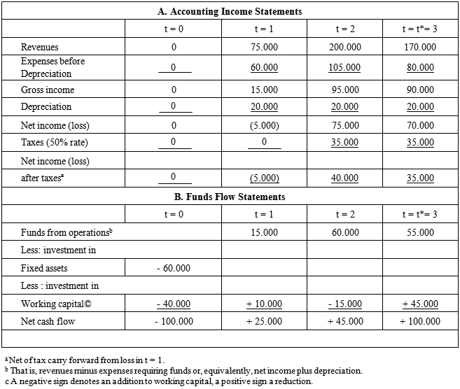And the development of the central idea underlies a large part of this volume. Our position is that the objective of financial management should be to maximize the value of the company to present shareholders.

In any case where value is determined by the DPV approach, the DPV notion of income is clearly the appropriate one. We should however, establish that different ways of looking at income and wealth result in substantially different ways of reporting the results of a given investment and cash-flow pattern. One such divergent method is the accounting process except to remark that basing income on historical data rather than expectations is antipodal to the notion of DPV- based income.

Another way in which wealth as monetary value can be viewed, which has a certain common-sense appeal, is based on the internal rate of return (IRR) basis for evaluating profitability. This method defines wealth as "owner-contributed funds plus the return on these funds as the internal rate of return less withdrawal." Specifically, for the same hypothetical company investing Io, assume that the return on this investment will be r> i.

Rather than working through all the implications of this notion formally, we will present a more or less realistic example of how the different interpretations of income would work out if applied to a hypothetical investment project.

Assume Io consists of a total outlay of $100,000, $60,000 of this for equipment (depreciated on a straight line basis) and $40,000 for working capital. The investment project will last three years, i.e., t* = 3. The tables above labelled A and B show accounting income and funds flow for the project. It is again assumed that cash returns on this investment are paid out to stockholders and not reinvested in the firm; also, the discount rate is set at i = 0.10 or 10%.

We can solve by using the following equation to obtain r = 0.25 or IRR = 25%

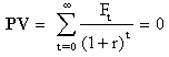Now, the table below sets out the figures obtained for income and wealth in period zero to period three, by applying the DPV, IRR, and accounting approaches. The DPV approach gives a windfall gain in t = 0 of $35,049 (later in my paper called pure profit); neither of the other approaches indicates that any income is realized during this period. Wealth, at the end of t = 0, is $135,049 where the DPV method is used, and $100,000 in each of the other cases. (Wealth is Vj in the DPV method, Ij in the IRR method, and the book value of equity in the accounting method).

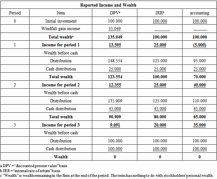Hint: Windfall gain income is the pure profit, I would explain it below under the concept of profit.

For the DPV method, the reported income in period 1 is $23,505 which is 10 per cent of the wealth at the beginning of that period. Since $25,000 is paid out to the shareholders, the value at the end of period 1 must be less than at the end of period 0, that is, $ 123,554 is less than $135,049. The income in period 2 is 10 per cent of $123,554 and so on.

Under the IRR approach, the wealth at the beginning of period 1 is $100,000, since the actual increase in the stockholders’ value is not reported. Income in this period is figured at 25 per cent of wealth, or $25,000. By chance, exactly this amount is paid out. Income in period 2 is 25 per cent of the remaining wealth, again $25,000, but in this case $45,000 is paid out, leaving a smaller base for period 3 income.

The accounting approach warns of a substantial loss in period 1, the accounting figures indicate substantially higher income in later periods.

HINT: Under the DPV approach as more and more of the project’s returns are paid out, the value of the stock declines, and consequently the income earned by the firm declines (even though the stockholders’ personal wealth may be continually increasing). Income figures obtained by other methods, however, do not follow this pattern and as a consequence, are not related in any simple way to the value of the firm’s stock.

The table below summarizes the income reported by the three methods. It will be noted that the total income reported over the three-year period is the same in every case only the timing of the reported income differs.

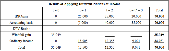This is not to say that alternate concepts of income may not be useful or necessary or both, but we must look at income from the shareholders’ point of view. This is the basic reason why the DPV approach is preferable.

3. A Theory of Cash-Flow

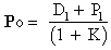
The Link between Stock Price and Net Cash-Flow:

A Cash-flow theory says that the value of the stock is the present value of the future net cash flows. And this Net Cash-Flow is the cash-flow between the firm and its stockholders. A positive net cash-flow represents a cash payment by the firm to the stockholders, while a negative net cash-flow represents a cash payment by the stockholders to the firm.

Example 1

Before going further in explaining the concept of “Cash-Flow Concept of Stock Valuation”, I would like to introduce a small example related to “Dividend Policy and Value” where I would show that the total value of the company depend on the Net Cash-flow between the firm and its stockholders and not on dividend :

First:

We already know that the value of a share of stock is established as the present value of all future dividends:

Second:

Assume that additional capital investment will be made at time one, but that all earnings will be paid out as dividends after that time. Then the value of a share of stock at time one is:

V1 is the value of the firm at time one

n is the number of shares outstanding at time zero

m is the number of shares that must be issued at time one to raise capital for predetermined new investments.

Then:

I1 is the amount of new equity required for capital investment at time one, so I1 = mP1, is a flow of cash from the stockholders to the firm.

Y1 is the amount of income at time one, and as all earnings are paid as dividends, so Y₁ = n D₁, is a flow of cash from the firm to the stockholders.

Then,

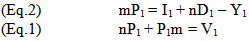If we substitute eq. 2 in eq. 1 we have the following:

nP₁ + (I₁ + nD₁ – Y₁) = V₁

nP₁ + nD₁ = V₁ – I₁ + Y1This equivalent to say P₁ = [(V₁ – I₁ + Y₁) / n] – D₁

Substituting P1 in the following Equation: Po = (P₁ + D₁) / 1 + K

Po = 【 [(V₁ –I₁ + Y₁) / n] – D₁ + D1】/ 1 + K

Simplifying Po = [(V₁ – I₁ + Y₁) / n] / 1 + K

V₁ is the present value at time one, predetermined set of investment.

I₁ is the amount of new equity required for capital investment at time one, a flow of cash from the stockholders to the firm. A negative sign.

Y₁ is the amount of income available at time one, a flow of cash from the firm to the stockholders. A positive sign.

n is the number of shares outstanding at time zero.

K is the required return for investment of this risk level.

The important thing to note is that dividends have disappeared ; the value of a share of stock have been defined by the net cash-flows determined as the flows between the firm and its stockholders, and that the Gordon Model used to find the value of a constant growth stock has become a cash-Flow theory of stock valuation.

These flows are not changed by the decision to finance internally or to issue new stock. If the stockholders receive a dividend of $1 million, this is a net cash-flow of plus $1 million. If $1 million of new stock is sold, this is a net cash flow of minus $1 million. If both transactions take place in the same period, the net cash-flow is the sum of the two, or zero. This is exactly what the net cash-flow would be if no dividends were paid, no new stock was issued, and the project was financed internally.

From here rises the cash-flow profit of stock valuation defined as the increase (decrease) in the stock value V1 plus the net cash-flow for the period (-I1 + Y1).

Example 2

Let us take another example to clarify and stress the cash flow concept of stock valuation, and let us make a shift from what was traditionally acceptable, “link between stock price and earnings “to “a link between stock price and cash-flows”.

This example is from the book of Brealy and Myers titled “Principles of Corporate Finance” chapter four.

Imagine the case of a company that does no grow at all. It does not plow back any earnings and simply produces a constant stream of dividends. Its stock would be rather like the perpetual bond and the return on perpetuity is equal to the yearly cash-flow divided by the present value. The expected return on our share would thus be equal to the yearly dividend divided by the share price (i.e., the dividend yield). Since all the earnings are paid out as dividend, the expected return is also equal to the earnings per share divided by the share price (i.e., the earnings-price ratio). For example, if the dividend is $10 a share and the stock price is $ 100, we have:

Expected return = Dividend yield = Earnings-price ratio

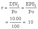The price equals

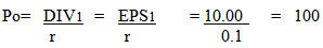The expected return for growing firms can also equal the earnings-price ratio. The key is whether earnings are reinvested to provide a return greater or less than the market capitalization rate. For example, suppose our monotonous company suddenly hears of an opportunity to invest $10 a share next year. This would mean no dividend at t=1. However, the company expects that in each subsequent year the project would earn $1 per share, so that the dividend could be increased to $11 a share.

Let us assume that this investment opportunity has about the same risk as the existing business. Then we can discount its cash flow at the 10 percent rate to find its net present value at year 1:

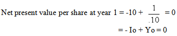What effect will the decision to undertake the project have on the company’s share price? Clearly none.

This could be explained in two different ways:

First: Trough a Link between stock price and Net Cash-Flows

Second: Trough a Link between stock price and Earnings

First: To explain the effect of the investment on the valuation of the firm according to the Net Cash-Flow Theory defined as the cash-flows between the firm and its stockholders for the period (- Io + Yo).

In our equation:

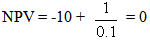
is the capital investment to undertake the project, a flow of cash from the stockholders to the firm, a negative sign.

is the amount of income the project would earn at time one discounted to time zero, a flow of cash from the firm to the stockholders, a positive sign.

The Net Cash-Flow is the sum of the two, or zero, this is exactly what will be the effect on the stock valuation.

Second: To explain the effect of the investment on the value of the firm according to the Earnings valuation. Brealy and Myers in their book said:

The investment opportunity will make no contribution to the company’s value because its prospective return is equal to the opportunity cost of capital. The reduction in value caused by the nil dividends in year one is exactly offset by the increase in value caused by the extra dividends in later years. Therefore, once again the market capitalization rate equals the earnings-price ratio:

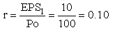The table below repeats our example for different assumptions about the cash-flow generated by the new project. Note that the earnings-price ratio, measured in terms of EPS₁, next year’s expected earnings, equals the market capitalization rate r only when the new project’s NPV = 0. This is an extremely important point; managers frequently make poor financial decisions because they confuse earnings-price ratios with the market capitalization rate.

Effects on stock price of investing an additional $10 in year 1 at different rates of return. Notice that the earnings-price ratio overestimates r when the project has negative NPV and underestimates it when the project has positive NPV.

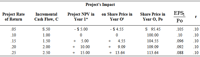In our last example both dividends and earnings were expected to grow at 10 percent, but this growth made no net contribution to the stock price. Be careful not to equate firm performance with the growth in earnings per share. A company that reinvests earnings at below the market capitalizations rate may increase earnings but will certainly reduce the share value.

In general, Brealy and Myers said in their book “Principle of Corporate Finance” That we can think of stock price as the capitalized value of average earnings under a no-growth policy, plus PVGO, the present value of growth opportunities:

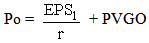The important thing to note here is that:

The first part of the equation is nothing than the discounted cash balance (V1) which will give its effect on the value of the stock.

The second components (PVGO) is nothing then the pure profit defined as the return in excess of the normal discount rate on invested capital (-Io + Y1).

So, under the Cash-Flow Theory of Stock Valuation, the price of the stock is determined by two components:

The First Component:

The first component is the present value of the future net cash-flows. Where management should project the future cash receipts and cash payments of the firm with various cash balances, subtract the payment from the receipts to determine net cash-flows, and then select that cash balance (i.e., purchase that amount of liquidity) which maximizes the present value of the net cash flows.

In a world of certainty it would be unprofitable for a firm to hold cash. Any cash not needed immediately to make payments would be lent at interest, as liquidity is worthless if all future cash needs can be perfectly foreseen, and there are no flotation costs associated with lending, borrowing or repaying money. In the presence of uncertainty, cash balances are held because they provide liquidity. In principle, the decision to purchase liquidity by increasing cash balances or to sell liquidity by reducing cash balances should be analysed in the same way any other investment decision is analysed. An increase in cash balances is therefore considered as a purchase of liquidity and is defined as a cash payment. A reduction in cash balances is a sale of liquidity and is defined as a cash receipt. If a firm receives cash from the sale of a product and increases its bank balance, this involves both a cash receipt and a cash payment, so that the net cash flow is zero. Subsequently, when the firm reduces its bank balance to pay wages, this is again both a cash receipt and a cash payment, with a net cash-flow of zero The net cash-flow in any period therefore is the difference between cash received by the firm from purchasers, debtors, or banks, and the cash used by the firm to increase cash balances, to pay for goods and services, to pay interest or repay debt, or to lend and such flows must be associated with equity valuation.

We could exclude all dealings in the firm’s financial obligations from the cash receipts and payments. The net-cash flow would then include transactions with debtholders as well as stockholders. The present value of the net cash flows would be the total value of all the firm’s financial obligations, and the value of the stock would be the total value of the obligations less the value of the debt. And this would provide the justification for the treatment of cash balances. cash balances are held because they provide liquidity. In principle, the decision to purchase liquidity by increasing cash balances or to sell liquidity by reducing cash balances should be analysed in the same way any other (investment) decision is analysed.

HINT: Management should project the future cash receipts and cash payments of the firm with various cash balances, subtract the payments from the receipts to determine net cash-flows, and then select that cash balances (i.e., purchase that amount of liquidity) which maximizes the present value of the net cash flow.

The net cash flow in any period therefore is the difference between cash received by the firm from purchasers, debtors, or banks, and the cash used by the firm to increase cash balances, to pay for goods and services, to pay interest or repay debt, or to lend. Such flows must be associated with equity obligations, i.e., the net cash flow is the cash flow between the firm and its stockholders. A positive net cash flow represents a cash payment by the firm to the stockholders, i.e., a dividend payment or a stock repurchase, while a negative net cash flow represents a cash payment by the stockholders to the firm, i.e., a new stock subscription.

The associated theory of stock valuation is based on the assumption that the cash receipts and the cash payments of the firm have been projected for each time period for ever. We assume that there are no transaction or flotation costs, or any costs other than interest (or dividends) involved in borrowing or repaying money, or in buying or selling financial obligations. We also assume that stockholders are indifferent between capital gains and dividend income, so that we would ignore problems which arise because of the different taxes on income and capital gains. The net cash-flow would then include transactions with debtholders as well stockholders. The present value of the net cash flows would be the total value of all the firm’s financial obligations, and the value of the stock would be the total value of the obligations less the value of the debt. So, that the present value of the net cash flows is the value of the stock. Since the peculiar treatment of cash balances does not arise in evaluating any decision except the decision about the level of cash balances themselves, our treatment of cash balances does not impair the usefulness of the cash-flow concept in investment decisions, but adds to its usefulness in stock valuation.

The associated theory of stock valuation is based on the assumption that the cash receipts and the cash payments of the firm have been projected for each time period for ever.

The Second Component:

The second component of the equation in order to be explained let us take an example of PVGO and link it to the cash flow concept of stock valuation. Let us turn to a well-known company, Fledging Electronics, Where its r, is 15 percent, the company is expected to pay a dividend of $5 in the first year, and thereafter the dividend is predicted to increase indefinitely by 10 percent a year. We can therefore, use the simplified constant-growth formula to work out Fledging’s price:

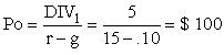Suppose that fledging has earnings per share of $8.33. Its payout ratio is then

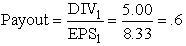In other words, the company is plowing back 1 - 0.6, or 40 percent of earnings. Suppose also that Fledging’ ratio of earnings to book equity is ROE = 0.25.This explains the growth rate of 10 percent:

Growth rate = g = plowback ratio × ROE =.4 ×.25 =.10

The capitalized value of Fledging’ earnings per share would be

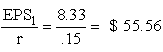But we know that the value of Fledging stock is $100. So, the question we can raise is, why investors are paying the difference of $44,44 per share. Let’s see if we can explain that figure:

Each year Fledging plows back 40 percent of its earnings into new assets. In the first year Fledging invests $3,33 at a permanent 25 percent return on equity. Thus the cash generated by this investment is 0.25 x 3,33 = $.83 per year starting at t = 2. The net present value of the investment as of t = 1 is

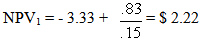Everything is the same in year 2 except that Fledging will invest $3,67, 10 percent more than in year 1 (remember g =.10). Therefore at t = 2 an investment is made

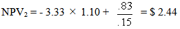These are the forecasted future cash-flow growing at 10 percent per year, to calculate their present value we use the simplified DCF formula,

Present value of growth opportunities = PVGO

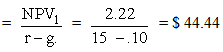Now everything checks:

Share price = present value of level stream of earnings + present value of growth opportunities

= + PVGO

Then, Po = $55.56 + $44.44 = $100

Why is Fledging Electronics a growth stock? Not because it is expanding at 10 percent per year. It is a growth stock because the net present value of its future investments accounts for a significant fraction (about 44 percent) of the stock’s price.

Here we have used the NPV to calculate this fraction of the stock’s price linked to the future cash-flow generated by the future investments of the firm.

Stock prices today reflect investors’ expectations of future operating and investment performance. Growth stocks sell at high price-earnings ratios because investors are willing to pay now for expected superior returns on investments that have not yet been made. Michael Eisner, the chairman of Walt Disney Productions, made the point this way: “In school you had to take the test and then be graded. Now we’re getting graded, and we haven’t taken the test. “This was in late 1985, when Disney stock was selling at nearly 20 times earnings. See Kathleen K. Weigner. “The Tinker Bell Principle,” Forbes, December 2, 1985, p. 102.

So, our second components - PVGO - is nothing then the pure profit or the concept of profit defined as the return in excess of the normal (discount rate) on invested capital. Cash-flow theory says that all pure profit is earned when the stock value makes a change that had not been anticipated by the market. The market value of the stock is always determined in such a way that the expected return, net cash-flow (dividends) plus capital gains, is the normal return on the market value at the start of the period. If all goes as expected, the actual return, business profit, will be the expected normal return, and pure profit will be zero. If expectation changes, a pure profit or loss is made immediately as the stock price makes an unexpected adjustment so that the newly expected future returns will equal a normal return on the new stock value (investment).

4. The Cash-Flow Concept of Dividend Policy

Although the problem of dividends were approached in a variety of ways, our preference said James E. Walter in his article on “Dividend policy and its influence on the value of the enterprise ” is to commence with net cash flows from operations and to consider the effect of additions to, and subtractions from, these flows upon stock values. Not only does this starting point by pass certain measurement problems, but it also directs attention to the relevant variables in a manner that other approaches may not. The question is whether dividends are in some sense of the word weighted differently from retained earnings at the margin in the minds of marginal investors.

Net cash-flows from operations are available for (1) the payment of interest and principal on debt or the equivalent and (2) capital expenditures and dividend payments. Operating cash flows can be supplemented in any period by debt or equity financing. Debt financing creates obligations to pay out cash in future periods and thereby reduces cash flows available for capital expenditures and dividend in those periods. Equity financing in turn, diminishes the pro rata share of total cash-flows available for dividends and reinvestment.

Before the thrust shifted to dividends, the basic issue in the cost of capital discussion was one of dividing the stream of operating cash-flows between debt and equity in such a manner as to maximize the market value of the enterprise. In an analogy to cost of capital, and when dividends enter the picture, the issue becomes one of dividing the stream of operating cash-flows among debt, dividends and reinvestment in such a way as to achieve the same result. The principal difference in the character of the analysis is that it may no longer be feasible to assume that the size and shape of the stream of operating cash-flows is independent of the manner in which it is subdivided.

Much the same as contractual interest payments and other financial outlays, the continuation of cash dividends at their prevailing rate is assigned a priority by management. In such instances, the burden of oscillations in operating cash-flows is placed upon lower-priority outlays, namely capital and related expenditures, unless management is both willing and able to compensate by adjusting the level of external financing. Even if management is willing to seek funds outside the firm, the uncertainties inherent in the terms under which external financing can be obtained in the future reduce the likelihood of such action in the event of operating cash deficiencies in any period. The reason is that current cash dividends may well be capitalized somewhat differently from anticipated future cash-flows.

It may be observed that the relative instability of expenditures designed to augment future cash-flows shows up even in the aggregate. The change from year to year for new plant and equipment averaged 19 percent for all manufacturing corporations in the post period to 1961, as compared with 9 percent for cash dividends. The maximum declines from one year to the next were 40 percent for new plant and equipment and but 2 percent for dividends.

Again, as in the case of debt versus equity, investor reactions to dividend policy changes can nullify in whole or in part their price effect. Whenever the stockholder is dissatisfied with the dividend payout, the balance between present and future income can be redressed by buying or selling shares of stock and perhaps by other means as well. for instance, by “lending” or “borrowing” on the same risk terms that cash dividends are paid. If dividends are deemed insufficient, the desired proportion of current income can be obtained by periodically selling part of the shares owned. If current income is too high, cash dividends can be used to acquire additional shares of stock. The one thing that shareholders cannot do through their purchase and sale transactions is to negate the consequences of investment decisions by management. If, as may well be the case, investment decisions tend to be linked with dividend policy, their neglect in the analysis of dividend effects seems inappropriate.

The conditions for no dividend effect under which changes in dividend payout have minimal influence upon stock values can now be stated. For the most part, they follow from the logics of stream-splitting:

The level of future cash-flows from operations, that is the growth rate, is independent of the dividend-payout policy. In essence, this condition implies that the impact of a change in dividend payout upon operating cash-flows will be exactly offset (or negated) by a corresponding and opposite change in supplemental (or external) financing. An increase in dividends can be offset only by the sale of equity shares. So, an increase in dividend payout will leave operating cash-flows unchanged in the aggregate, but the share of future cash-flows accruing to existing stockholders will decline, since additional stock has to be sold to finance the planned capital outlays. The existing shareholder can, of course, reconstitute his former pro rata position by purchasing shares in the market with his incremental dividends.

Implicit in these remarks is the presumption that the market completely capitalizes anticipated growth in operating cash-flows. New shares are thus acquired at a price that returns new investors only the going market rate for the relevant class risks. The present value of extraordinary returns from investment by the corporation goes to existing stockholders, rather than to new shareholders. To the degree that the anticipated level of operating cash-flows, that is, the growth rate, is connected with the dividend payout for one reason or another, the market value of the firm may be conditioned by variations in dividend payout. The policy changes may be unexpected, and their price effect lies at least upon the relation between the internal and market rates of return. If the former exceeds the latter, the present value of a dollar employed by the firm (other things being equal) will be greater than a dollar of dividends distributed and invested elsewhere. This issue was considered in 1956 paper by James E. Walter. From here rises a Cash-Flow Concept of Stock Valuation where the value of the stock is the present value of the future net cash-flows. And this Net Cash-Flow is the cash-flow between the firm and its stockholders; a positive net cash-flow represents a cash payment by the firm to the stockholders, while a negative net cash-flow represents a cash payment by the stockholders to the firm. The question that arises here is, do the weights employed or in other words, the discount factors, independent of the dividend-payout policy? Provided that the system of weights remains unchanged, a change in current cash dividends will alter the stockholder’s stake in future cash-flows.

According to the question of the independence of the weights used from the dividend-payout policy, a change in dividend payout undoubtedly disturbs the investors in that stock to some extent unless the modification was anticipated previously. Insofar as costs of one kind or another and other factors prevent the shareholders thus activated from completely reconstituting their old position and thereby give rise to a new and different equilibrium point. The fact that the substitutions of future cash-flows for present dividends superimposes an element of market risk upon the basic uncertainty of the operating cash-flow stream. As contrasted with cash dividends in which the stockholder receives a dollar for each dollar declared, there is no telling what price the shareholder will realize in the market at any given time for his stake in future cash-flows. From here rises the need for a theory of stock pricing based on cash-flow analysis.

A recent article by John Lintner, concludes that “generalized uncertainty “ is itself sufficient to insure that shareholders will not be indifferent to whether cash dividends are increased or reduced by substituting new equity issues for retained earnings to finance given capital budgets.

The frequently observed association between dividend-payout policy, capital structure, and rate of growth is a useful case in point. The survival of the corporation ordinarily does not depend; in the short run at least, upon any specific rate of growth. The prime considerations affecting growth, apart from profit opportunities, are (1) the willingness of corporations to go into the public market place for additional funds and (2) their attitude toward dividends, including their willingness to return unneeded funds to the investors.

For firms that are reluctant to get involved in external financing, and there appear to be many, then the burden of expansion rests upon residual internal sources, that is, operating cash-flows less cash dividends and debt servicing net of additions to debt. Decisions to increase or decrease dividends thus condition the value of the enterprise as long as the returns on new investments differ from the market rate. Whenever the available investment opportunities are unable to earn their keep, the specter of liquidating, dividends or repurchase of shares or debt retirement arises. If there is no debt outstanding and if the repurchase of shares is not contemplated, the burden of liquidation falls upon dividend payout.

So, we can conclude that we should have a look not on the dividend effect on the value of the enterprise but on the effect of cash-flow from operation on stock valuation, because and if the change in the level ( increase or decrease ) of dividend would affect the future cash-flow from operation not necessary on the aggregate, but on the share of future cash-flows accruing to existing stockholders. This must have its effect on the value of the stock and indirectly we should discount the (decrease - increase) in the cash-flow from operation and compare it to the discounted (decrease or increase) in cash dividend, and find out the net effect on the price of the stock. This would bring us back to our definition of the cash-flow concept of stock valuation where the net cash-flow when discounted will have its effect positively or negatively on the value of the enterprise and this Net Cash-flow is nothing than the flow of cash between the firm and its stockholders.

5. The Cash-flow Concept of Stock Valuation and the Cost of Capital

To solve the problem of the calculation of the cost of capital or the cost of equity or the required rate of return by the shareholders or the implicit cost. Let us have a look on the benefit of the net cash-flow.

We would show in this part that depreciation and implicit cost need not be considered since they don’t give rise to cash-flows. Cash-flow analysis accounts for these costs much more simply, by charging the cost as a cash payment when the asset is bought.

Calculating Project NPV:

Maple Media is considering a proposal to enter a new line of business. In reviewing the proposal, the company’s CFO is considering the following facts:

The new business will require the company to purchase additional fixed assets that will cost $600,000 at t = 0. For tax and accounting purposes, these costs will be depreciated on a straight-line basis over three years. (Annual depreciation will be $200,000 per year at t = 1, 2, and 3.)

At the end of three years, the company will get out of the business and will sell the fixed assets at a salvage value of $100,000.

The project will require a $50,000 increase in net operating working capital at t = 0, which will be recovered at t = 3.

The company’s marginal tax rate is 35 percent.

The new business is expected to generate $2 million in sales each year (at t = 1, 2, and 3). The operating costs excluding depreciation are expected to be $1.4 million per year.

The project’s cost of capital is 12 percent.

What is the project’s net present value (NPV)?

Solution:

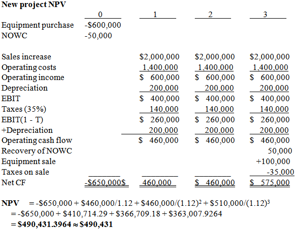Let us now calculate the Economic profit. Then calculate the discounted present value of the economic profit:

Economic profit = Earnings – Cost of equity

Hint: Equity is decreased every year by the depreciation

Year 1 = $260 000 – ($650 000 x 12%) = $182 000

Year 2 = $260 000 – ($450 000 x 12%) = $206 000

Year 3 = $260 000 – ($250 000 x 12%) = $230 000

PV of Economic profit = $182 000/ 1.12 + $206 000 / (1.12)² + $230 000 / (1.12)³

= $490 431.39 ≈ $490 431

We conclude that the discounted economic profit is equal to the discounted cash-flow or the Net Present Value (NPV). The important thing to notice is that Depreciation and implicit interest need not be considered since they do not give rise to cash flows. Cash-flow analysis accounts for these costs much more simply by charging the cost as a cash payment when the asset is bought.

This come to emphasize what have been already challenged by Professors Biddle, Bowen, and Wallace in their article “EVA and its Critics” in the Journal of Applied Corporate Finance, Summer 1999.Where they argue that Cash-flow from operations, accruals and interest expense, are already included in the profits numbers that companies are required to disclose in their annual reports. The question is whether or not the two elements not explicitly included in mandated disclosures, the capital charges and accounting adjustments are significantly related to stock prices. Unhappily the answer is NO. They show that while the cash-flow and actual components are consistently significant, the components unique to EVA are not.

In our example we excluded the salvage value. What about if we add the salvage value to our calculation:

NPV = -$650,000 + $460,000/1.12 + $460,000/(1.12)² + $575,000/(1.12)³

= -$650,000+$410,714.29+$366,709.18 + $409,273.64

= $536,697.11 ≈ $536,697.

Under the discounted economic profit we consider the salvage value as a cash payment from the firm to the shareholders and in our case it is equal to:

Equipment sale $ 100 000

Taxes on sale $ (35 000)

PV (Economic profit) = $182000/1.12+ $206 000 /(1.12)² + $230 000 /(1.12)³ + $ 65 000 /(1.12)³

= $536 697.1119 ≈ $536 697

The important thing to notice is that Depreciation and implicit interest need not be considered since they do not give rise to cash flows. Cash-flow analysis accounts for these costs much more simply, by charging the cost as a cash payment when the asset is bought.

5.1. Debt or Equity Financing under the Cash-flow Theory of Stock Valuation

If we continue with the same example of Maple Media Corporation using debt financing, we will find out that the discounted present value of the economic profit using debt financing is always equal to the Net Present Value meaning that the way of financing is not affecting the value of the firm as long as the net cash-flow is not changing. We will have access to reducing debt financing only when the net cash-flow is decreasing in order to reduce the effect of reduction on the net cash-flow on the value of the firm.

Though capital structure decisions are influenced by a firm’s ability to generate future cash flows, the theoretical literature has neglected the dynamic relation between leverage and firm specific earnings behaviour. HOWEVER, with the cash-flow theory of stock valuation, under a theory of continuous time, we have adjustments in the business, capital structure, policy and optimality on hour per hour and day per day basis in order to avoid the risk inherent in the capital structure of the business. We will use the article of Steven Raymar “A Model of Capital Structure when Earnings are Mean-Reverting” to give a clear meaning to a theory of continuous time. Raymar assumes a linkage between firm value and earnings, which would affect the optimal leverage decisions. So, leverage is reviewed and reoptimized every period and the variability of leverage is positively related to variability in earnings and firm value. EBIT follows an exogenous process that is unaffected by leverage or default. Its parameters are such that the firm never liquidates if optimal policies are followed. The autocorrelation between earnings at time t and t+1 is , if =0, earnings are serially independent, and as approaches 1 the process tends toward a random walk, implication of the process is that, while a firm may experience a bad or a good year, over time it is expected to revert to a normal performance level. An unlevered firm is valued as the discounted sum of expected future after-tax earnings, because stockholders receive the firm’s income stream in perpetuity, it must never be optimal for them to relinquish ownership, as it might be if income were negative, this would be optimal for stockholders to maintain the unlevered firm as a going concern, given any feasible earnings realization. When debt is introduced in the financing activities of the corporation, the firm is assumed to issue single period debt and to optimally recapitalize at each date.

As firm optimally and continuously recapitalize, under continuous time the focus is not on conflicts of interest among claimants, because debt has a one period maturity, the optimal policy should maximize both equity and firm value, so adjustments are made on daily basis and when earnings are low, a firm should optimally reduce its leverage ratio and debt level or otherwise said reducing its cost of capital and the earnings process permits one firm to be safer than another over a short horizon. At each date, the firm is recapitalized so as to maximize the wealth of current owners. This process is costless if the firm is solvent, but otherwise the transfer of ownership and control is assumed to induce bankruptcy reorganization costs and the model is unaffected as long as a clear distinction between debt and equity remains. Default that caused liquidation in the past is now resulting in an optimal reorganization. Since an optimal debt decision needs to consider only the future cash-flows of the firm and is independent of past earnings and debt levels. Then a change in the autocorrelation between earnings at time t and t+1, also affects future debt decisions and firm values. From here rises a cash-flow concept of profit associated with the cash-flow theory of stock value.

6. The Traditional Performance Measures

The problems and the effective performance measures like Return on Asset (ROA), Return on Equity (ROE), Return on Investment (ROI) and Economic Value Added (EVA), and how these measures correlate positively with stock-returns and stock prices, will be discussed below.

6.1. Problems with Return on Equity (ROE)

We said that managers should strive to maximize shareholder wealth. If a firm takes steps to improve its ROE, does it mean that shareholder wealth will also increase? Not necessarily, for despite its widespread use and the fact that ROE, and shareholder wealth are often highly correlated, some problems can arise when firms use ROE as the sole measure of performance.

First, ROE does not consider risk. While shareholders clearly care about returns, they also care about risk. To illustrate this point, consider two divisions within the same firm. Divisions S, has very stable cash flows and a predictable 15 percent ROE. Division R, on the other hand, has a 16 percent expected ROE, but its cash-flows are very risky. If mangers were compensated solely on the basis of ROE, and if the expected ROEs were actually achieved, then Division R’s manager would receive a higher bonus than Division S’s manager, even though Division S may actually create more value for shareholders as a result of its lower risk.

Second, ROE does not consider the amount of invested capital. To illustrate this point, let’s consider a rather extreme example. A large company has $1 invested in Project A, which has an ROE of 50 percent, and $1million invested in Project B, which has a 40 percent ROE. The projects are equally risky, and the two returns are both well above the cost the company has to pay for the capital invested in the projects. In this example Project A has a higher ROE, but since it is so small, it does little to enhance shareholder wealth. Project B, on the other hand, has the lower ROE, but it adds much more to shareholder value.

Consider one last problem with ROE. Assume that you manage a division of a large firm. The firm uses ROE as the sole measure of performance, and it determines bonuses on the basis of ROE. Toward the end of the fiscal year, your division’s ROE is an impressive 45 percent. Now you have an opportunity to invest in a large low-risk project that has an estimated ROE of 35 percent, which is well above the cost of the capital you need to make the investment. Even though this project is profitable, you might be reluctant to make the investment because it would reduce your division’s average ROE, and therefore reduce the size of your year-end bonus.

These three examples suggest that a project’s return must be combined with its risk and size to determine its effect on shareholder value. To the extent that ROE focuses only on rate of return, increasing ROE may in some cases be inconsistent with increasing shareholder wealth. With this in mind, academics, practitioners, and consultants have tried to develop alternative measures that overcome ROE’s potential problems when it is used as the sole gauge of performance.

Thus the level of ROE does not tell the owner if the company is creating shareholders wealth or destroying it. Thus ROE is an informative measure and can’t be used to decision making or to guide operations.

6.1.1. How Is ROE Connected To EVA?

To better understand the idea behind EVA and how it is connected to ROE, Let us look at Keller Electronics, Keller has $100,000 in operating capital, which in turn, consists of $50,000 of common equity and $50,000 of long-term debt. The company has no preferred stock or notes payable. The long-term debt has a 10 percent interest rate. However, since the company is in the 40 percent tax bracket, and interest expense is tax deductible, the after-tax cost of debt is only 6 percent. On the basis of their assessment of the company’s risk shareholders require a 14 percent return. This 14 percent return is what shareholders could expect to get if they were to take their money elsewhere and invest in stocks that have the same risk as Keller. Keller’s overall cost of capital is a weighted average of the cost of debt and equity, and it is 10 percent, found as 0.50(6%) + 0.50(14%) = 10%. The total dollar cost of capital per year is 0.10($100,000) = $10,000.

Now let us look at Keller’s income statement. Its operating income EBIT, is $20,000, and its interest expense is 0.10($50,000) = $5,000. Therefore its taxable income is $20,000 - $5,000 = $15,000. Taxes equal 40 percent of taxable income, or 0.4($15,000) = 6,000, so the firm’s net income is $9,000, and its return on equity, ROE, is $9,000/$50,000 = 18%

Now what is Keller’s EVA?

EVA= EBIT (1 - Corporate tax rate) – (Operating capital x After-tax percentage cost of capital)

= $20,000(1-0.4) – ($100,000)(0.10) = $2,000

This $2,000 EVA indicates that Keller provided its shareholders with $2,000 more than they could have earned elsewhere by investing in other stocks with the same risk as Keller’s stock. To see where this $2,000 comes from, let’s trace what happens to the money:

• The firm generates $20,000 in operating income.

• $6,000 goes to the government to pay taxes, leaving $14,000.

• $5,000 goes to the bondholders in the form of interest payments, thus leaving $9,000.

• $7,000 is what Keller’s shareholder’s expected to earn:

0.14($50,000) = $7,000.

Note that this $7,000 payment is not a requirement to stay in business, companies can stay in business as long as they pay their bills and their taxes. However, this $7,000 is what shareholders expected to earn, and it is the amount the firm must earn if it is to avoid reducing shareholder wealth.

• What is left over, the $2,000, is EVA. In this case, Keller’s management created wealth because it provided shareholders with a return greater than what they presumably would have earned on alternative investments with the same risk as Keller’s stock.

• We said that EVA is different from the traditional accounting measure of profit in that EVA explicitly considers not just the interest cost of debt but also the cost of equity. Indeed, using the simple example above, we could also express EVA as net income minus the dollar cost of equity:

EVA = Net income – [(Equity capital) (Cost of equity capital)]

= $9,000 – [($50,000)(0.14)]

= $2,000

Note that this is the same number we calculated before when we used the formula for calculating EVA. Note also that the expression above could be rewritten as follows:

EVA = (Equity capital) [(Net income / Equity capital) – Cost of equity capital]

Or simply as:

EVA = (Equity capital) (ROE – Cost of equity capital)

This last expression implies that EVA depends on three factors: rate of return, as reflected in ROE; risk, which affects the cost of equity; and size, which is measured by the amount of equity capital employed.

6.1.2. Problem with Return on Net Assets (RONA)

The return on net assets (RONA) is calculated as follows:

RONA = NOPAT / net assets

Net assets = Cash + Working Capital Requirement + Fixed Assets

Working Capital Requirements = (Receivables + Inventories + Prepayments) – (Short- term non-interest bearing liabilities).

Why not using RONA by itself?

The risk to companies of using RONA, is that divisional managers might bypass value creating projects because they would reduce RONA (a risk whenever RONA is greater than WACC), or they might undertake value destroying projects because they would increase RONA (which can happen when RONA is less than WACC). Either way, reliance on RONA alone can lead to suboptimal behaviour.

The balance sheets shown below clarify how invested capital is defined:

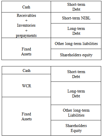The balance sheet on the left is a normal balance sheet. On the right we see a balance sheet in which short-term non-interest-bearing liabilities are netted against short-term operating assets – inventories, receivables, and prepaid expenses. The left side of this balance sheet is referred to as “net assets”; “invested capital” appears on the right side.

The latter problem was a serious risk in Japanese companies. Few large Japanese firms have earned large RONAs in recent years, and with the country’s recent economic downturn, the situation has worsened. The average RONA in 1997 for large publicly traded Japanese companies was practically zero. Still growing capital market pressure has led several of these companies to adopt RONA or return on equity (ROE) as a measure of corporate performance. If managers of these companies are evaluated on RONA, and RONA is significantly lower than WACC, which it is for most large Japanese companies, managers might be tempted to invest in capital projects that will earn less than the WACC as long as they are expected to earn more than the existing RONA. The result is that value-destroying Japanese companies may invest ever-increasing amounts of capital in value-destroying activities, digging themselves, and the Japanese economy, into an ever-deeper hole.

A few years ago, Apple Computer faced a very different problem. Its managers too, were evaluated on the basis of RONA. Moreover, as recently as the early 1990s, the company’s RONA was 30 percent, among the highest of any large American business. This high RONA made management reluctant to make further investments, passing up opportunities with expected returns of 20 percent despite the fact that these returns far exceeded the company’s cost of capital. The result is that Apple systematically underinvested, contributing to the massive problems that brought the company to the brink of the collapse in 1997. Choosing the wrong measure to focus on certainly didn’t help. We invest whenever the returns are expected to exceed the cost of capital.

Still RONA is a major improvement over the measures that companies have normally relied on to measure performance. We learned this lesson firsthand from work with a well-known German manufacturer. This company had invested heavily over a period of several years in new plant and equipment. Senior managers congratulated themselves on the resulting improvements in employee productivity that showed steady growth in output per employee. To these managers, this meant that the company has achieved huge efficiency gains. Yet they were puzzled by the company’ mediocre financial performance. On closer inspection, it became clear that what the company had really accomplished was the substitution of labour with new but capital-intensive technologies. Output per employee grew, but the company’s output charts conveniently ignored the huge increase in capital that made the output gains possible. Employees had become more “efficient,” but only at the expense of lower asset and capital efficiency.

An important virtue of RONA is that it not only captures any productivity gains achieved by the company’s workforce, but it also considers the assets the workforce uses to achieve its output. Although it does not explicitly measure capital charges, it does remind managers that there is a cost to acquiring and holding assets.

6.2. Problems with Economic Value Added

Economic Value Added was developed and popularized by the consulting firm Stern Stewart & Co., EVA helps managers ensure that a given business unit is adding to stockholder value, while investors can use it to spot stocks that are likely to increase in value. What exactly is EVA? EVA is a way to measure an operation’s true profitability. The cost of debt capital (interest expense) is deducted when calculating net income, but no cost is deducted to account for the cost of common equity. Therefore, in an economic sense, net income overstates “true” income. EVA overcomes this flow in conventional accounting.

Surprisingly, many corporate executives have no idea how much capital they are using or what that capital costs. The cost of debt capital is easy to determine because it shows up in financial statements as interest expense. However, the cost of equity capital, which is actually much larger than the cost of debt capital, does not appear in financial statements. As a result managers often regard equity as free capital, even though it actually has a high cost. So, until a management team determines its cost of capital, it cannot know whether it is covering all costs and thereby adding value to the firm.

Although EVA is perhaps the most widely discussed concept in finance today, it is not completely new; the need to earn more than the cost of capital is actually one of the oldest ideas in business. However, the idea is often lost because of a misguided focus on conventional accounting.

The basic formula for EVA is as follows:

EVA = Net operating profit after taxes, or NOPAT – After-tax dollar cost of capital used to support operations

EVA = EBIT (1- Corporate tax rate) – (Operating capital) x (After-tax percentage cost of capital).

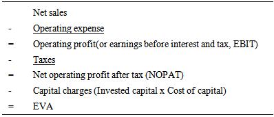Operating capital is the sum of the interest-bearing debt, preferred stock, and common equity used to acquire the company’s net operating assets, that are its net operating working capital plus net plant and equipment. Operating assets by definition equals the capital used to buy operating assets.

EVA is an estimate of a business’s true economic profit for the year, and it differs sharply from accounting profit, the most important reason EVA differs from accounting profit is that the cost of equity capital is deducted when EVA is calculated. Other factors that could lead to differences include adjustments that might be made to depreciation, to research and development costs, to inventory valuations, and so on.

EVA represents the residual income that remains after the cost of all capital, including equity capital has been deducted, whereas accounting profit is determined without imposing a charge for equity capital. Equity capital has a cost, because funds provided by shareholders could have been invested elsewhere where they would have earned a return. Shareholders give up the opportunity to invest funds elsewhere when they provide capital to the firm. The return they could earn elsewhere in investments of equal risk represents the cost of equity capital. This cost is an opportunity cost rather than an accounting cost.

Note that when calculating EVA we do not add back depreciation. Although it is not a cash expense, depreciation is a cost, and it is therefore deducted when determining both net income and EVA. Our calculation of EVA assumes that the true economic depreciation of the company’s fixed assets exactly equals the depreciation used for accounting and tax purposes. If this were not the case, adjustments would have to be made to obtain a more accurate measure of EVA.

An Alternative to Accounting-Based EVA: The Refined EVA (REVA).

There is an approach to calculating EVA that reduces reliance on accounting conventions. In this version of EVA, invested capital is based on the market value of the firm, instead of the book value of invested capital. Although NOPAT is still based on GAAP under this approach, invested capital is not. In this way, its advocates assert, the relationship between EVA and share price significantly improves.

To understand the nature of this argument, consider an example:

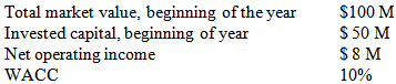When conventionally measured, based on beginning invested capital, EVA equals $3 million [$8 million – ($50 million x 10 percent)]. Critics argue, however, that the firm’s $100 million market value implies that its capital providers would have expected a $10 million return ($100 million x 10 percent) had they invested their funds elsewhere. Therefore, as the argument goes, if the company is to create value in that year, it must generate a return greater than $10 million. In this case, despite a positive EVA of $3 million, net operating income is obviously not sufficient to earn an acceptable return on capital. The problem stems from the measurement of capital, which is based solely on the assets in place and ignores the net present value of future investment opportunity (which may be priced by the market but ignored on the balance sheet).

The proposed solution is a modified version of EVA that its creators call refined EVA (or REVA). Under REVA, capital charges are based on the market value of the firm, and not the market value of the firm, and not the adjusted book value approach. In this example, REVA equals a negative $2 million [$8 million – ($100 million x10 percent )], which is more consistent with the company’s performance that year from the shareholders’ perspective and more highly correlated with stock market returns than conventional EVA. But because it is measured from market values, and market values are usually available only at the firm wide level, REVA can be used only at the corporate level. EVA would still be needed at lower levels of the organization. The problem with REVA results from confusing market values, which incorporate expectations of future performance for the long-term, with single-period measures of operating performance.

Consider the case of Coca-Cola. Suppose Coca-Cola has a market value of $150 billion at the beginning of the REVA measurement period. If its WACC is 10 percent, capital charges total $15 billion. These days, even outstanding performance by the company in the coming year –say, a NOPAT of $5 billion, will yield a REVA of negative $10 billion! Does this mean that the company destroys value? Probably not. It is quite possible, indeed even probable, that Coca-Cola can produce NOPAT of $5billion (and a negative REVA of $10 billion) and still cause its share price to increase because the $5 billion of NOPAT in the current period is higher than what the market expected. The market may then reasonably interpret this performance to indicate that even more EVA will be generated in the future than was expected before Coca-Cola’s results were known. In other words, even if REVA is hugely negative, which is always the case for the most successful value creators, the implications of the current year’s performance for future EVAs could result in a higher share price. How then do we interpret a negative REVA?

One of REVA’s creators has privately conceded this point to us but argues that the measure’s real value is detecting mispriced securities and not as a measure of corporate performance. Companies with highly negative REVA stocks would be viewed as overpriced. While highly positive REVA stocks would be viewed as under-priced. The problem with this logic is that nearly all companies with large EVA growth expectations impounded in their existing share price will have a negative REVA. Are all, or even most, such companies overpriced?

Under the REVA approach, invested capital is measured on the basis of total market value, including the capitalized value of future growth opportunities. Meanwhile, NOPAT is based entirely on current operating performance, ignoring, as does any short-term financial measure, the value-creating effects of investing activities, such as R&D, that may deliver huge amounts of EVA in the future.

If a company is systematically creating future growth value, its capital charges under REVA will increase from one year to the next. For Coca-Cola, the company’s huge market value at the beginning of the period ($150 billion) is a result of its success in previous periods of creating FGV. In other words, the company has been highly successful in convincing the capital markets that future EVAs will be much higher than historical EVAs. Perhaps the company has created valuable strategic options that are expected to translate into outstanding financial results in the future. While the value of these options is reflected in market value, it will not, and cannot, be reflected in REVA. In short, REVA will always ignore value-creating activities that are not reflected in the current year’s operating results, while charging management for a capital base that includes the capitalized value of such activities from previous years.

Coke’s REVA may be -$5 billion, implying massive underperformance, but because it created valuable growth opportunities that year, shareholder values was created, not destroyed. The irony of REVA is that those companies that are most successful in creating future growth opportunities, and therefore the companies with the highest excess returns, will have the lowest and most negative REVAs.

6.2.1. Problem with Return on Investment (ROI) and the Discrepancy in Accounting Rate of Return and EVA

Every project that a firm undertakes should have positive Net present value (NPV) in order to be acceptable from the shareholders point of view. This means that a project should have internal rate of return bigger than the cost of capital. With practical performance measuring the internal rate of return cannot be measured and some accounting rate of return is used instead to estimate the rate of return to capital. Typically this rate of return is some form of return on investment (ROI). Unfortunately, any accounting rate of return cannot on average produce an accurate estimate of the underlying true rate of return. Although EVA is a value based measure, and it gives in valuations exactly same answer as discounted cash flow, the periodic EVA value still have some accounting distortions. That is because EVA is after all an accounting based concept, suffering from the same problems of accounting rate of returns (ROI). In other words, the historical asset values that distort ROI distort EVA values as well. The following formula shows that EVA is based on the accounting return.

EVA = (ROI-WACC)*CAPITALEMPLOYED

Unfortunately accounting rate of return has at least two severe pitfalls: first, wrong periodising meaning EVA is divided unevenly between different years. With normal depreciation schedules, EVA and ROI tend to be small at the beginning of a project and big at the end of the project. Therefore companies with a lot of new investments have lower EVA than their true profitability would imply. Second, distortions caused by inflation and asset structure. Historical asset values are distorted by inflation which affects also EVA values. As proved many times in financial literature, accounting rate of return is also unable to describe the true rate of return even with no inflation. The extent of this problem depends on the asset structure (the relative proportions of current assets, depreciable assets, un-depreciable assets) and on the length of investment period.

Moreover, the change in assets structure during one investment period might increase or decrease wrong periodising. For example, if a company has a lot of new assets, and new investments, it is likely to have low ROI compared to true rate of return due to the change of assets proportion from the beginning to the end of the investment period.

Other than the problem of wrong periodising, ROI is a poor measure of a company’s true rate of return due to inflation. When the difference between accounting ROI and IRR. Salmon and Laya proved this inflation effect in 1967 and De Villiers discussed it in 1976, and it is well documented in economic literature. In addition to inflation, the duration of the project and the assets structure affects the discrepancy between ROI and IRR, the longer the duration of the project the higher the difference between the two rates. These discrepancies when they exist, they affects EVA since it is calculated from the accounting based figures. EVA overstates shareholders value if ROI overstates IRR. In order to decrease the discrepancies, De Villiers suggested in 1997 to adjust EVA by using current value of assets and capital in calculating accounting rate of return (ROI) (Makelainen, 1998).

6.2.2. The Effectiveness of EVA in Management Bonus Plans and its Correlation to Share Prices

According to the EVA theory the market value of a company is, its book value plus the current value of future EVA:

Market Value of Equity =Book Value of Equity + Present value of all future EVA.

This relationship between EVA and the market value of a company suggests that EVA drives the market values of shares. Studies made on the American and European companies in the late eighteens concluded that EVA correlates positively with stock returns and this correlation is slightly better than with traditional performance measures like return on assets, return on equity, and return on sales. They also conclude that EVA is an effective measure that contains information about the quality of strategic decisions and change to be taken by management. Stern Stewart & Co. made a study on 100 bank holding companies data between 1986 and 1995. They found that the correlation between some performance measures and market share to be as follows: EVA 40%, ROA13%, ROE 10%, and earnings per share 6%. Moreover, companies which went on EVA have noticed increase in its Market value added (MVA) and noticed an increase in share prices. Lehn and Makhija (1996) study EVA and MVA as performance measures and signals for strategic change. Their data consists of 241 U.S. companies and cover years 1987, 1988, 1992 and 1993. The researchers first find out that both measures correlate positively with stock returns and that the correlation is better than with traditional performance measures like return on assets (ROA), return on equity (ROE) and return on sales (ROS). Additionally they study how companies’ performance, measured in terms of EVA and MVA, effect on the CEO firings. Finally they examine the relationship between EVA/MVA and corporate focus. Lehn and Makhija find an inverse relation between EVA/MVA and abnormal CEO turnover. They also find that firms with greater focus on their business activities have significantly higher MVA than their less focused counterparts. Lehn and Makhija conclude that their results suggest EVA and MVA to be effective performance measures that contain information about the quality of strategic decisions and serve as signals of strategic change.

The idea of EVA bonuses is that if management can be paid some bonuses, shareholders would be better off, earning higher return on their capital than they expect. Thus, it would be beneficial for both management and the shareholders, because performance measure will rise when introducing EVA bonus system (Wallace 1997). Wallace (1997) studied the effects of adopting management bonus plans based on residual income measures. The sample in the study consists of forty firms that have some residual income measure, mainly EVA, as bonus base. This sample was compared to sample of same size consisting of similar companies where the bonus is tied to accounting based measures. Wallace tests with various methods the management actions in these sample groups and concluded that the results as being consistent with a residual income-based performance measure providing incentives for managers to act more like owners, thus mitigating the inherent conflict between managers and shareholders.” The firms that adopted residual income based compensation outperformed the market over the twenty-four month period by over 4% points in cumulative terms.

EVA bonus system is considered as a motivating bonus system that encourages managers to exceed the normal performance level. Bonus can be paid according to some percentage of positive EVA or according to some percentage of improved EVA. Thus managers have incentives to maximize performance and value of their corporation.

EVA bonus systems are also good in decreasing agency problems. And with this system managers avoid investments that produce less than WACC and also avoided investing in not so good projects, because when producing a return less than WACC decrease the bonuses. Therefore, EVA bonus systems unite the interest of group management and shareholders or the interest of group and managers.

In addition, EVA bonus system is a way to pay employees according to the change in productivity. Thus EVA bonuses could bring some elasticity in the payroll of workers, and avoid some oversized wage increase demands.

Implementing EVA in a company requires of course some kind of management effort. However, if right actions are taken straight from the beginning then implementing EVA should be one of the easiest changes that a company goes through. The actions required by management include the following: first, gaining the understanding and commitment of all the members of the management group through training and discussing. Managers should know exactly what EVA is all about and what differences there are compared to other measures like EPS and ROI. CEO and all the divisions’ managers should communicate their support and believe in the concept to the whole company. Second, training of the other employees, especially all the key persons in every department because they are the ones who use it operationally, and their understanding of the concept is essential in bringing EVA downwards to all company levels. Third, adopting EVA in all levels of organization should not be only a tool for management. EVA is powerful at operational levels to illustrate the costs of working capital, inventories, sales, receivables etc… to operating employees like sales people, operating engineers and others. EVA approach helps employees to see how costly capital is. EVA can be calculated by producers and by customers in every day’s operations. Fourth, integrating EVA as a bonus incentive plan for all employees, EVA bonus system helps employees to struggle for the common goal of which is increasing shareholder value.

EVA became a popular performance measure despite its suffering from some accounting distortions like ROI. It helps understanding the cost of capital of a company and it gets employees and managers to think and act like shareholders. Moreover, they start to consider that long-term investments produce at least a return that covers the most of capital otherwise shareholders will be better off investing elsewhere. Management should not operate with lazy or excess capital and should aim in to create shareholders value by enlarging the spread between return and cost of capital multiplied by capital employed. Capital tied to operations should be minimized. The idea is to cut excess capital and not only to cut costs. The power of EVA approach is that studies fail to trace the correlation between EVA and share prices but at the same time they can prove that EVA is better correlated to share prices than other traditional performance measures.

In order to achieve high EVA, managers should be trained to act and think like owners. EVA bonus plans give managers interest in performance improvements by paying bonuses that are a fixed percentage of all changes in EVA. This EVA bonus plan should have four objectives: First, giving managers motivation and compensation to choose strategic decisions that maximize shareholders value. Second, train and motivate managers to work long hour, take risks that some managers would take during industry downturns and recessions, fourth, to keep shareholder costs at a reasonable level (Stewart, 2002).

As a performance measure in corporate world, EVA helps the management and also other employees to understand the cost of equity capital mainly in big public companies, which do not have a strong owner, shareholders have often been conceived as a free source of funds. Similarly, business unit managers often seem to think that they have the right to invest all the retained earnings that their business unit has accumulated although the group would have better investment opportunities elsewhere. EVA might change the attitude in this sense because it emphasizes the requirement to earn sufficient return on all capital employed.

Including capital costs in the income statement helps everybody in the organization to see the true costs of capital. When calculating EVA, the cost of equity and debt can be subtracted in the income statement earlier than after the net operating profit.

At best EVA can be a new approach to view business. Perhaps the biggest benefit of this approach is to get the employees and managers to think and act like shareholders. It emphasizes that in order to justify investments in the long run they have to produce at least a return that covers the cost of capital. In other case the shareholders would be better off investing elsewhere. This approach includes that the organization tries to operate without lazy or excess capital and it is understood that the ultimate aim of the firm is to create shareholder value by enlarging the product of positive spread between return and cost of capital multiplied with the capital employed. The approach creates a new focus on minimizing the capital tied to operations. According to Wallace study (1996), companies using EVA had gained superior-performance.

6.2.3. The main Problems with EVA in Measuring Operating Performance are

EVA is poor in periodising the returns of a single investment. It underestimates the return in the beginning and overestimates it in the end of the period. Some growth phase companies or business units have a lot of new investments. Such growth phase companies are likely to have currently negative EVA although their true rate of return would be good and so their true long-term shareholder wealth added true long-term EVA would be positive. Also EVA suffers from other distortions including failing to estimate the value added to shareholders, because of the inflation and other factors. That is also the reason why EVA is criticized to be a short-term performance measure.

It certainly holds also more generally that EVA or any other financial performance measure do not in itself provide managers with sufficient information. Financial measures tell us the outcome of many different things. They usually hide the causes of good or bad profitability. The good or bad performance of individual processes is seldom visible in financial performance measures. Some other measures pinpoint the current situation of critical success factors much better. Therefore every company should use many measures in estimating how their plans are going and strategic goals are reached.

The new famous concept called Balanced Scorecard (Kaplan & Norton 1996) presents that companies should use several different perspectives in measuring performance to avoid the distortions of EVA. The perspectives suggested are (Kaplan & Norton 1996):

• Financial (How should we appear to our shareholders?)

• Customer (How should we appear to our customers?)

• Internal Business Process (To satisfy our shareholders and customers, what business processes we must excel at?)

• Learning and growth (To achieve our vision, how will we sustain our ability to change and improve?)

Professors Kaplan and Norton present that in order to fulfil financial objectives set by shareholders, the company should concentrate on besides financial measures also on measures of the other perspectives. If a company has measured customer perspective well and reacted in it with operations (internal business process perspective), the result is often improved financial performance. Financial measures do not often show the reasons but the consequences. Therefore it is utmost important to have also other measures. Sometimes focus on EVA and shareholder value is incorrectly viewed as opposite approach to Balanced Scorecard. On the contrary Professors Kaplan and Norton (1996) present that EVA is one suitable and widely used financial performance measure for financial perspective. According to Kaplan and Norton (1996) the financial perspective is the critical summary and the main goal. It must not be neither over nor underemphasized. “A failure to convert improved operational performance in the Scorecard, into improved financial performance should send executives back to their drawing boards to rethink the company’s strategy or its implementation plans.” (Kaplan & Norton 1996). In the end, every strategic plan has to convert into long run profitability in order to be justified.

A good example of the necessity of different measures is provided with the browser and other Internet software producer Netscape. The company did huge losses in its early years but still it was viewed as valuable company because of the expected big positive future cash flows.

The Problems with EVA is that, EVA is distorted by ROI due to underestimating the return in the beginning and overestimating it in the end of the project period especially in the case of a single investment. Some companies that have many investments in the beginning will have a current negative EVA but the ROI will be good compared to IRR, hence their true long term shareholder wealth added would be positive. Ceasing investments can increase short term EVA and that is why EVA is criticized to be a short –term performance measure. Companies focusing on long term investments that do not occur in a continuous stream showed no interest in EVA.

Another short sightedness is that the true EVA of long term investments cannot be measured objectively because future returns cannot be measured but can be subjectively estimated. The only subjective component to be used in EVA model is the depreciation schedule. In addition, the problem of wrong periodising and its effect on long term results should be considered. This problem should be solved in case all investments proved to be really profitable as ROI approaches IRR. It can be expected that companies with a lot of new undepreciable assets have negative EVA in the near future and that is why companies have invested heavily today and expect positive cash flow in a distant future, are considered extreme examples and EVA is not a primary performance measure for them. One example would be telecommunication operators who heavily invest in infrastructure with very long- term payoffs.

Another problem is that EVA measure tells us if the outcome is good or bad and whether value is added or reduced but it hides the causes of this outcome, so more measures should be taken by one company to understand more its strategic goals. Finally, as ROI fails on average to estimate the true return, EVA fails on average to estimate the value added shareholders due to inflation and assets structure and project duration. Using the current value of assets instead of book value is the solution (Ehbar, 1998).

EVA is an effective method for teaching workers. The first measure is to change managers behaviour, making them thinks and act like owners. Most important, it is a good analysis tool and a good internal motivation system for managers and employees for the best performance possible (Ehrbar, 1998).

6.2.4. Stock Market Returns: Is EVA Beating Earnings or Is Cash-Flow Really Better?

Professors G.C. Biddle, R. M. Bowen, and J. S. Wallace in their article “Does EVA Beat Earnings? “Evidence on Associations with Stock Returns and Firm Values” Journal of Accounting & Economics, December 1997, pp. 301-336, who argue that earnings have more explanatory power than EVA. The Biddle, Bowen, and Wallace study provides evidence on the information content of EVA, residual income (i.e., unadjusted EVA), net income (before extraordinary items), and cash-flow from operations. Information content describes the relation between the measure in question and changes in stock prices. The first question addressed is whether EVA (either in its adjusted or unadjusted form) dominates net income and cash-flow from operations in explaining annual stock market returns. When they look at a large sample of firms covering the period 1984 to 1993, the authors find R square for net income of 12.8 percent, versus 7.3 percent for residual income (i.e., unadjusted EVA), 6.5 percent for EVA (the adjusted version), and 2.8 percent for cash-flow from operations. In other words, annual accounting earnings had nearly twice the power of EVA in explaining one-year stock returns. The authors then extended the study to include five-year return intervals. Again, accounting earnings did better with R square of 31.2 percent, versus 18.9 percent for cash-flow from operations, 14.5 percent for EVA, and 10,9 percent for residual income. The differences in explanatory power between net income and each of the three other performance measures are highly significant for both the one-year and the five-year intervals. The authors even segmented the sample for firms known to have adopted EVA and those that had not, on the assumption that firms may adopt EVA at least in part because their past experience indicates a strong relation between EVA and stock returns. Also investors may become more attuned to EVA and, therefore, more likely to incorporate it in pricing shares for companies that announce they are adopting it. Alas, EVA still fails to outperform earnings, although earnings no longer dominate EVA.

The study then addresses whether components unique to EVA or residual income help to explain stock returns beyond that explained by net income and cash-flow from operations. The logic behind this test can be seen below:

EVA = CFO ± Accruals + After-tax interest expense – Capital charges ± Accounting adjustment

Cash-flow from operations is embedded in net income. The difference between the two figures is a function of accrual accounting. Depreciation, deferred taxes, and receivables are examples of items that cause cash-flow from operations and net income to diverge. In short,

Cash-flow from operations (+) or (–) the various elements of accrual accounting equal net income. Adding after-tax interest expense back to net income produces a measure of unlevered profit, or NOPAT. Residual income is calculated by subtracting capital charges capital charges from NOPAT. The difference between residual income and EVA is caused by the various adjustments. These adjustments are added to or subtracted from residual income to produce EVA. The first three elements in the EVA calculation – cash-flow from operations, accruals, and interest expense – are already included in the profit numbers that companies are required to disclose in their annual reports. The question the authors seek to answer is whether or not the two elements not explicitly included in mandated disclosures – capital charges and accounting adjustments – are significantly related to stock prices. Unhappily, the answer is no. They show that while the cash-flow and accrual components are consistently significant, the components unique to EVA are not.

Still, the Biddle, Bowen, and Wallace results are not entirely persuasive. One problem is that their regression analysis seems to show that while investors put great weight on the cost of debt, the cost of equity is apparently ignored. For more extensive critique of the Biddle, Bowen, and Wallace study, see S.F. O’Byrne, “EVA and its Critics,” Journal of Applied Corporate Finance, Summer 1999. The independent variables in these regressions are current and prior period values for each of the five EVA components shown in the figure below: CFO, accruals, after-tax expense, capital charges, and accounting adjustments.

The coefficients tell us that an additional dollar of cash-flow from operations adds $2.128 to the five-year return, while an additional dollar of capital charge subtracts $0.088. This implies that $24 of capital charge (or $2.128/$0.088) is needed to offset the economic benefit of $1 of cash-flow from operations, which suggests that investors are virtually indifferent to capital costs. This is a far cry from EVA, which reminds us of what should be an obvious fact - $1 of capital charge offsets the economic benefit of +$1 of earnings.

Table 1. Shows the coefficients for the regression on five-year stock returns, where the independent variables are five-year sums

However, a more careful look at the regression coefficients shows that capital costs matter a good deal more than the capital charge coefficient suggests. The regression obscures the impact of capital costs because it does not fully separate financing and operating performance. Cash-flow from operations includes after-tax interest expense. This means that current period after-tax interest expense appears in the regression three times as a negative component of the capital charge ; and as a separate independent variable. This implies that the aggregate coefficient on current period after-tax interest expense is –2.735 (or –2.128 + -0.509 + -0.088). This in turn, has two very puzzling implications. First, it implies that $1.29 (or $2.735/$2.128) of positive cash-flow from operations is needed to offset the economic cost of $1 of after-tax interest expense. Since after-tax interest expense is computed using the statutory corporate tax rate, one explanation for this odd differential is that the effective tax saving is less than the statutory rate. Second, and much more puzzling, it implies that $1 of after-tax interest expense has the same economic cost as 31 (or $2.735/$0.088) of equity capital cost.

This is an odd result, because it suggests that equity capital is basically free. Biddle, Bowen, and Wallace may have overlooked the issue raised by after-tax interest expense because they expected the after-tax interest variable to have a negative sign. It should have a positive sign in the regression, just as it does in the EVA components equation, since after-tax interest expense is adding back the expense buried in cash-flow from operations.

The problem with the accounting adjustments proposed for the calculation of EVA is not that they are illogical. In some circumstances, adjustments are necessary. For example, in cases where retail companies lease nearly all their assets and thus keep them off the balance sheet, meaningful EVA figures require that leases be capitalized, even if GAAP says differently. Still for most companies, the assumption of zero adjustments is a logical starting point in deciding how EVA is to be measured.

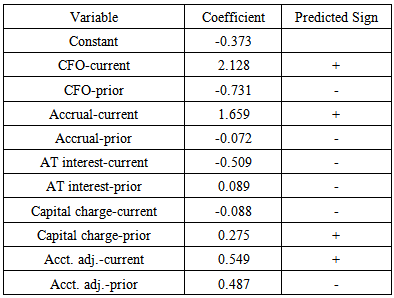
7. From Economic Value Added (EVA) to the Cash-Flow Concept of Stock Valuation

Let us take the following example to show the link between the Economic Value added and the cash-flow concept of stock valuation. This example, we are able to see is a very simple model of the business. Adding hired labour and raw materials to the model makes it a bit more complex, but the lesson still holds. Here then, is the problem:

In 1/1/ X, we buy a business for $250,000. We pay &100,000 of our own money (Which we could have “invested” elsewhere at 10 %), and borrow $150,000 from a bank, on which we pay a 10 % interest rate. At that point, my balance sheet shows Assets of $250,000; Liabilities of $150,000, and a Net Worth of $100,000. To focus on the issues at hand, let us suppose the business is extremely simple. Specifically, we have no outlays on raw materials or hired labour, and we don’t supply any of our own labour or entrepreneurial services. Over the course of the year, suppose we receive revenue of $47,000 and pay out bank interest of $15,000. Also suppose the value of our physical assets (machines building and tools) decreases by $17,000, from $250,000 to $233,000. Then our economic income statement is very simple:

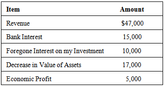Remember that economic profit is calculated by subtracting total economic cost from total revenue. Total economic cost, in turn, is the sum of explicit cost and implicit cost.

Explicit cost is the outlays the firm makes for resources that are used up during the year.

In this example, the only explicit cost is bank interest. Implicit costs are forgone inflows. Because the owners’ resources are put to use in this firm, instead of their best alternative use, those owners are not able to obtain the flow of dollars they would get in the alternative use (Of course, the reason the resources are put in this use is that the owners expect to get more here.). In this example, implicit cost (foregone interest plus “economic depreciation”) is $27,000 ($10,000 plus $17,000). Thus total economic cost is $42,000, and economic profit (total revenue minus total economic cost) is $5,000.

What we want to show is that the $5,000 economic profit represents the amount by which we are richer than we would have been if we had deployed our resources ( in this case, our $100,000) in their best alternative use rather than in this business. What would my position have been if we had invested our $100,000 in our best alternative instead of in this business? We started with $100,000 on 1/1/X, and that amount would have grown to $110,000 by 12/31/X if invested at 10% our assumed opportunity in our best alternative investment vehicle. What is my situation in this business? We can determine that by looking at our new balance sheet:

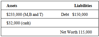Notice the asset item for $32,000 (cash). This comes from the fact that we received $47,000 in Total Revenue during the year, but only paid out $15,000 in bank interest. The remainder is assumed to have gone into our bank account. The M, B and T asset reflects the “true economic depreciation” in their value from $250,000 to $233,000 over the year. We also assumed that we paid only the interest due on our bank loan. The key thing to notice is that we are $5,000 wealthier because we bought and operated this business than we would have been if we had invested our $100,000 in our best alternative. (It would be easy to put items for supplying our own labour, hiring other labour, and buying raw materials, but they would only complicate the story at this point, without giving us any new insights).

Now how the results could be seen under the cash-flow concept of stock valuation:

We already know that Pure Earning P1 is equal to:

P1 = N1 – D1 + B1 + rNo( here No is a negative number because it is a flow of cash from stockholders to the firm ).

P1 = Pure earning in year one

N1 = $32,000 (Cash-flow generated in year one).

D1 = $17000 (Depreciation expense)

B1 = Zero (Current Debt repayment)

rNo= 10% ( $-100,000) (Cost of Equity Capital)

P1 = $32,000 - $17,000 +0 – $10,000 = $5,000 which is the EVA calculated above, and which is the pure profit which is above the normal profit of 10% of the beginning investment by shareholders at the start of the year, leading to the following new balance sheet under the cash-flow concept of stock valuation:

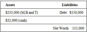The expected increase in net worth was 10% out of the $100,000 the initial investment of shareholders at the beginning of the period. However an increase in wealth of $5,000 was created to shareholders:

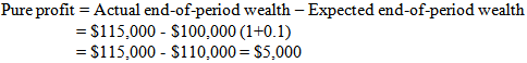
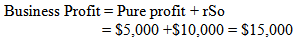How would things be different if we looked at them in an accounting framework?

Accounting profit is calculated by subtracting total accounting cost from revenue. Accounting cost, in turn, is equal to explicit costs plus what might be called a “capital consumption allowance,” or accounting depreciation. The accounting measure of depreciation will usually differ from economic depreciation. Remember that economic depreciation is the actual decrease in the market value of the firm’s assets over the year. By any of contrast, accounting depreciation is calculated by using the original purchase price, the assumed life of the asset, and a salvage value at the end of its life, and some rule or formula for allocating the difference between the original purchase price and the salvage value over the assumed life of the asset.

Accounting cost can differ from economic cost (and accounting profit can differ from economic profit) both because the two approaches measure depreciation differently and because accountants do not attempt to measure foregone inflows, such as interest that the owners could have earned if they had invested their funds elsewhere (or, in a more complicated example, wages that a proprietor could have earned if he had been employed elsewhere instead of running his own business).

In this story, accounting profit is simply revenue ($47,000) minus bank interest paid ($15,000) minus accounting depreciation. Let’s suppose that accounting depreciation is $20,000. Then accounting profit is $12,000. What does this tell us? Since the calculation does not ascertain what the resources that are being used in this firm could have done elsewhere. It could be that owners are happy earning what they earn here or unhappy, but there is no way of knowing just from looking at the accounting profit number. By way of contrast, economic profit tells owners at a glance what they want to know, namely whether they are doing better here than they would in their best alternative employment. If economic profit is positive, they are doing better here than they could anywhere else. If economic profit is negative even if accounting profit is positive, owners’ resources would be able to earn more in their best alternative employment than they could here. If economic profit is zero, owners are doing exactly as well here as they could in their best alternative employment. Thus, if owners of a firm could get an accurate measure of economic profit, they would know whether or not they could increase their wealth by leaving this business.

What we claim in economics is that, if decision-makers are interested in increasing their wealth, they should make decisions using economic profit, because that number will tell them whether they are in the right business. But since that number is inherently subjective, this means that business decisions must necessarily be subjective. Decision-makers must make a subjective judgment about what the owners ‘resources could earn in their best alternative use and what the firm’s assets could be sold for today and in the future.

In our example, suppose that accounting depreciation equalled economic depreciation ($17,000). Then accounting cost would be $32,000, and accounting profit would be $15,000. The only difference between economic cost and accounting cost is now that economic cost counts the amount the owners could have earned by investing elsewhere as a cost, whereas accounting cost does not include this item. By adding to accounting cost an item for forgone interest, we can get an approximation to economic cost. In this case, that foregone interest (calculated by multiplying the return owners could earn elsewhere by the amount they could have cleared by selling out at the beginning of the year) is $10,000. Subtracting that $10,000 from the year’s accounting profit gives us our measure of economic profit, $5,000.

While it can be useful for a decision-maker to know whether the firm made an economic profit over the past year, the way economists use economic profit is always forward-looking. That is, we assume decision-makers decide what to do (for example, whether to stay in this business) by trying to estimate the resources supplied by owners can be better here than in their best alternative, that is, they try to estimate whether the firm will make an economic profit, an economic loss, or break-even economically in the future.

However, in the cash flow concept of stock valuation we have shown that the depreciation and implicit interest need not be considered since they don’t give rise to cash-flow. And the present value of the pure earnings is the present value of the net cash-flows.

The differences between the cash-flow profit approach and the traditional earnings approach can be illustrated by the analysis of a simple investment project. The project requires a capital outlay of $1000 at the beginning of the first year. At the end of the first year the firm will receive $1120 in sales revenue and will pay $400 in wages and $60 in corporate income taxes. At the end of the second year the firm will receive $1310 in sales revenue and pay $500 in wages and $205 in corporate income taxes. The income taxes are calculated by charging $600 of depreciation expenses the first year and $400 the second, which we assume the tax laws to permit. A 50 percent tax rate is then applied to taxable income (revenue minus wages minus depreciation) of $120 the first year and $410 the second year. No other receipts or payments are associated with the project.

The project therefore has a net cash-flow of -$1000 at the start of the first year, +$660 at the end of the first year and +$605 at the end of the second year. If we assume a discount rate of 10 per cent, the present value of the net cash flow is +$100 for the project.

Now let us see the implications of the cash-flow analysis of this project with its associated profit and stock values if we assume that an entrepreneur incorporates solely for the purpose of engaging in this project, and that this project is equity financing by assuming a net cash-flow of -$1000 when the asset is purchased. By definition, a net cash-flow is a transaction with stockholders, and the negative sign implies a flow of cash from the stockholders to the firm. The simplest case to consider is one in which the investment project was not anticipated by the market, but the market adopts the firm’s forecast of the future net cash-flows immediately when the asset is purchased.

1. An entrepreneur takes $1,000 of his own money and buys an asset with the expectation that he can get a net cash flow of $660 at the end of the first year, and $605 at the end of the second.

2. He incorporates and issues stock to himself at the same time that he buys the asset.

3. The market values of the stock is at $1100 when it is issued, because this is the present value of the expected future cash-flows, discounted at 10 per cent.

4. The entrepreneur therefore makes a capital gain of $100 at the time that he issue the stock since he has paid $1,000 for the asset and has stock which he can liquidate for $1100. This increase in his wealth takes place whether or not he actually sells the stock, and in his “initial investment” in the firm. It is also a business profit, and a pure profit, received at the start of the first year, since his actual wealth is $1100, and his expected (by the market) wealth had been $1000.

5. If all goes as expected, the firm returns $660 to its stockholders at the end of the first year. If the expectations for the second year are unchanged, the stockholders also have stock valued at $550, which is the present value of the cash flow of $605 expected at the end of the year. The stockholders’ actual end-of-period wealth is $660 + $550 = $1210, and business profit is $110 in the first year. Pure profit is zero since the stockholders’ normal 10 percent rate of return on their initial investment of $1100 is also $110.

6. If expectations continue to be realized, the firm returns $605 to its stockholders at the end of the second year, and the stock becomes worthless. End-of-period wealth is therefore $605. The initial investment for the second year is $550 since this is the stock value at the start of the year. Business profit is therefore $55 and pure profit is still zero.

Cash-flow theory says that all pure profit is earned when the stock value makes a change that had not been anticipated by the market. The market value of the stock is always determined in such a way that the expected return, net cash-flow (dividends) plus capital gain, is the normal return on the market value at the start of the period. If all goes as expected, the actual return, business profit, will be the expected normal return, and pure profit will be zero. If expectations change, a pure profit (or loss) is made immediately as the stock price makes an unexpected adjustment so that the newly expected future returns will equal a normal return on the new stock value (investment).

Analysis of the project within the context of traditional earnings theory requires information about economic depreciation which cash-flow analysis does not require. Cash-flow analysis requires only information about corporate income taxes, which requires knowledge about legal depreciation but not about economic depreciation (another way of looking at this is to observe that no depreciation calculation would be required for cash-flow analysis if there were no income tax, while depreciation would still be required for earnings analysis). While there is some debate, particularly among accountants, about the precise meaning of economic depreciation, we shall assume that it is the change in the market value of the asset. We can assume, for the time being, that legal depreciation and economic depreciation are the same, i.e, that the asset has a value of $400 at the end of the first year. Traditional earnings analysis then says that the firm raises $1000 in capital at the start of the first year. It earns (net of taxes) $60 the first year. Since it returns $660 at the end of the year, $600 of this represents a return of capital, and the stockholders still have $400 invested. The second year earnings are $205. Since $605 is paid to stockholders at the end of the year, this represents a disbursement of the earnings and a full return of the $400 investment.

In the table below we can summarize the cash-flow and the earnings analysis:

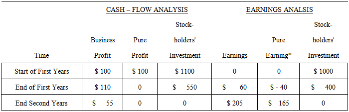Since the discount rate is 10% we have

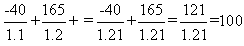Cash-flow analysis therefore shows an immediate capital gain of $100, with subsequent business profits of a normal 10% on investment and no pure profit. Earnings analysis shows no immediate capital gain, earnings of 6% on investment the first year and 51% the second year.

We now turn to the discussion of the reasons for preferring the cash-flow approach:

First, the depreciation problem,

The fundamental criticism of the treatment of depreciation in earnings analysis is that the economic depreciation expense understates the capital costs involved. The actual cost is $1000 at the start of year one, while the depreciation expenses over the two years add (undiscounted) to $1000. The present (start of year one) value of the depreciation expenses is therefore less than the actual cost of $1,000. (This criticism applies to long-run static equilibrium where depreciation just covers replacement in each period so that the initial investment never gets charged as an expense. Let the initial investment be I, with annual replacement of R. The present value of the investment plus replacement is therefore I + R/r. If the annual depreciation charge is D, the present value of the depreciation charges is D/r. In long-run static equilibrium D=R, and the true cost of investment, I+R/r, exceeds the present value of the depreciation expenses by the initial investment, I.).

The solution to this problem, within the framework of earnings analysis, is to charge an implicit interest expense on the book value of the stockholders’ investment (net worth) at the normal rate of return, 10%. In the case of equity financing which we have been considering, this is equivalent to charging implicit interest on the undepreciated asset balance. However, if the asset is financed in whole or in part by debt, this of course, would change the net cash flows. In our example, if $500 is raised by debt borrowing the net cash flow at the start of the first year is only -$500. There is a cash payment of $1000 for the asset and a cash receipt of $500 from debtholders. Only $ 500 is raised from stockholders, and this is the net cash flow. The net cash flows would be reduced in subsequent periods also, because debt repayment and interest are cash payments which must be subtracted from the cash receipts to get the cash flows (to stockholders). The debt financing might also raise the discount rate on the equity return (net cash-flow), but we continue to assume that the appropriate discount rate, as influenced by the debt issue, is known. In this case interest is included explicitly; cost would be overstated by including an implicit interest expense on the entire undepreciated asset balance.

The inclusion of implicit interest on net worth makes the present (start of first year) value of the costs charged to equity capital in each year, depreciation minus debt repayment plus implicit interest, equal to the initial equity investment. Since the present value of the debt repayment and associated interest expenses must equal the initial debt investment, all capital charges are accounted for.

To justify this point please follow the example below:

Consider a case in which the net cash flows are N_o at the start of the first year, N₁ at the end of the year N₂ at the end of the second years. Bonds (B) are issued at the start of the first year, of which B₁ are due at the end of the first year and B-B₁ at the end of the second year. The initial asset value is A = B-N_o, since we raise N_o from stockholders. Depreciation is D₁ the first year and A-D₁ the second year. The book value of the net worth is-N_o at the start of the first year, so the implicit interest charge is- rN_o. The firm returns N₁ to its stockholders at the end of the first year, of which N₁-D₁ + B₁ represent earnings and D₁-B₁represent a return of capital. Book value of net worth is therefore, –No-D₁ + B₁ at the end of the first year, and implicit interest of r(-N_o-D₁ + B₁) must be charged in the second year. Charges (C) against equity capital are depreciation minus debt retirement plus implicit interest. So we have:

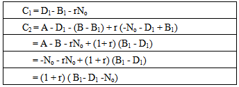We can now define pure earnings as earnings minus implicit interest, and pure earnings then account for all capital costs. In our example, the book value of the stockholders’ investment is $1000 at the start of the first year and $400 at the start of the second, so implicit interest would be $100 the first year and $40 the second, and pure earnings account for capital costs means that the present (start of first year) value of the pure earnings is the same as the present value of the net cash-flows, which also account for all capital costs.

Let us use the table below to justify our finding:

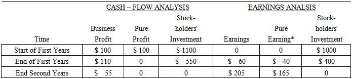Since the discount rate is 10 % we have

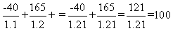More generally, denoting the pure earnings by

P₁ and P₂, we have

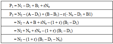Cash-flow analysis accounts for these costs much more simply, however, by charging the cost as a cash payment when the asset is bought. Depreciation and implicit interest need not be considered since they do not give rise to cash flows.

Second, the maximization problem,

The correct calculation of capital costs is necessary for decision making. This means that the maximization of earnings is not in the stockholders interest, while the maximization of pure earnings is.

The maximization of earnings can be misleading even in the determination of the output rate by setting marginal cost equal to marginal revenue in the framework of comparative statics. In this case the marginal revenue is the same as the marginal cash receipts and marginal cost is the marginal cash payment so that the difference between marginal revenue and marginal cost is the marginal net cash-flow. Since a positive marginal net cash-flow necessarily increases the present value of the future net cash-flows and so increases profits, cash-flow theory confirms the traditional result that output should be increased if marginal revenue exceeds marginal cost.

This is true, however, only if both revenues and costs increase at the same time. If the cost increases first and sometime elapses before the product is sold and revenue increases, then the cash outlay during this time interval must be regarded as an investment in the context of earnings analysis or as a net cash payment in the context of cash-flow analysis. Earnings will rise if marginal revenue exceeds marginal cost, but the output should be increased only if the difference is large enough to provide a normal rate of return on the additional (equity) investment, so that earnings maximization is an inadequate decision criterion. Cash-flow analysis gives the correct result by requiring that the present value of the future net cash receipts generated when the marginal revenue exceeds marginal cost be at least as large as the present value of the net cash payments generated after the marginal cost has risen but before the marginal revenue has risen.

An example related to the investment project discussed in the last section will illuminate some of the problems. Suppose that a firm must select either that project or an alternative project which has identical cash flows, but which has economic depreciation of $500 in each of the two years. Such a project would be indistinguishable from the first using cash-flow analysis. Earnings analysis, however, would show earnings of $160 the first year (instead of $ 60 as the original project) and of $105 the second year (instead of $ 205). Pure earnings would be $60 the first year (instead of -$40) and $55 the second year (instead of $165). Earnings maximization would lead to the selection of the alternative project, since it earns $100 more the first year and $100 less the second year. Maximization of pure earnings, however, again leads to the conclusion that the projects are equally profitable since the present value of the pure earnings is $100 for either project.

This is not a coincidence and illustrates a very important point. The present value of the pure earnings of a project does not depend in any way on the economic depreciation pattern, even though the economic depreciation is charged as an expense in the various periods. We have already seen that the present value of the pure earnings equals the present value of the net cash-flows, and neither the net cash-flows nor their present value is influenced by the pattern of economic depreciation. The conclusion is that earnings maximization is not an appropriate decision criterion unless the earnings are corrected for implicit interest on the book value of the net worth to obtain pure earnings. The present value of the pure earnings, however, is independent of the depreciation pattern so that it hardly seems worthwhile to go to the trouble of determining depreciation and the implicit interest charge. It is simple (but logically the same) to maximize the present value of the net cash flows.

Third, the timing problem,

The only possible advantages of pure earnings over cash-flow profit would be either that they give a more accurate picture of the timing of the benefits from the investment project, or that they are more easily measurable at the end of the period.

With respect to timing, cash-flow theory says that the original project creates a pure profit of $100 at the start of the first year, and then earns only a normal 10 per cent profit on investment in the next two years. Earnings theory says that there are no pure earnings at the start of the first year, that the return on investment during the first year falls short of a normal 10 per cent return by $40 (pure earnings of -$40) and exceeds a normal 10 percent return by $165 during the second year. Since the present (start of first year) value of the pure earnings is the same as the present value of the pure profit, the dispute is really about the timing of the realization of the pure profit or earnings, not about the total amount involved.

The approaches agree in defining pure profit as the ordinary profit (Which we call business profit) or earnings less a normal return on invested capital. They differ both in their measurements of the ordinary profit or earnings and in their measurements of the ordinary profit or earnings and in their measurement of the amount of invested capital.

If we adopt the strongest version of traditional theory and value assets at market, so that depreciation is the change in market value, then both cash-flow and traditional theory base their measurements of profit (or earnings) and invested capital on market values. Earnings are associated with the potential sale of the firm’s assets at market value. Cash-flow profit is associated with the potential sale of the firm’s equities at market value.

Traditional earnings are the difference between the book value of the net worth at the end of the year and book value at the beginning of the year, plus the net cash flow. It is associated with asset values because the net worth is the residual when debt is subtracted from the market value of the assets. It therefore shows the gains accruing to the stockholder because the firm refrained from selling its assets at market for an additional year. Cash-flow business profit is the difference between the market value of the stock at the end of the year and its market value at the beginning of the year also plus the net cash-flow. It therefore shows the income accruing to stockholders because they held their stock for an additional year, if we define income in the usual way as that maximum possible consumption without reducing wealth.

The traditional approach is to measure the stockholders’ investment as the book value of the net worth, and we have already seen that this is the appropriate base in the determination of implicit interest. Cash-flow theory measures the stockholders’ investment as the market value of the firm’s stock.

Fourth, the measurement problem,

If the objective of the firm is to earn a profit for its stockholders, the amount of profit earned during a period can be used as a criterion in measuring the performance of the firm. It is therefore desirable to have a profit concept which can be measured on the basis of market values, so the measurement will be objective in the accounting sense.

Of the four profit concepts we have considered, two, business profit and earnings, are measurable from market data. Neither pure earnings nor pure profit is so measurable since they both require the use of the normal rate of return and this is not directly observable in the market. As earnings maximization is not in the stockholders’ interest, it is not a satisfactory measure of performance. This leaves business profit as the only satisfactory measure of performance.

8. The Net Cash-flow Theory of Stock Valuation is the Daily Cash Transaction between the Firm and Its Stockholders

The present value of the future net cash-flows where management should project the future cash receipts and cash payments of the firm with various cash balances, subtract the payment from the receipts to determine net cash-flows, and then select that cash balance (i.e., purchase that amount of liquidity ) which maximizes the present value of the net cash flows.

In a world of certainty it would be unprofitable for a firm to hold cash. Any cash not needed immediately to make payments would be lent at interest, as liquidity is worthless if all future cash needs can be perfectly foreseen, and there are no flotation costs associated with lending, borrowing or repaying money. In the presence of uncertainty, cash balances are held because they provide liquidity. In principle, the decision to purchase liquidity by increasing cash balances or to sell liquidity by reducing cash balances should be analysed in the same way any other investment decision is analysed. An increase in cash balances is therefore considered as a purchase of liquidity and is defined as a cash payment. A reduction in cash balances is a sale of liquidity and is defined as a cash receipt. If a firm receives cash from the sale of a product and increases its bank balance, this involves both a cash receipt and a cash payment, so that the net cash flow is zero. Subsequently, when the firm reduces its bank balance to pay wages, this is again both a cash receipt and a cash payment, with a net cash-flow of zero The net cash-flow in any period therefore is the difference between cash received by the firm from purchasers, debtors, or banks, and the cash used by the firm to increase cash balances, to pay for goods and services, to pay interest or repay debt, or to lend and such flows must be associated with equity valuation.

We could exclude all dealings in the firm’s financial obligations from the cash receipts and payments. The net-cash flow would then include transactions with debtholders as well as stockholders. The present value of the net cash flows would be the total value of all the firm’s financial obligations, and the value of the stock would be the total value of the obligations less the value of the debt. And this would provide the justification for the treatment of cash balances, cash balances are held because they provide liquidity. In principle, the decision to purchase liquidity by increasing cash balances or to sell liquidity by reducing cash balances should be analysed in the same way any other (investment) decision is analysed. HINT: Management should project the future cash receipts and cash payments of the firm with various cash balances, subtract the payments from the receipts to determine net cash-flows, and then select that cash balances (i.e., purchase that amount of liquidity) which maximizes the present value of the net cash flow.

The net cash flow in any period therefore is the difference between cash received by the firm from purchasers, debtors, or banks, and the cash used by the firm to increase cash balances, to pay for goods and services, to pay interest or repay debt, or to lend. Such flows must be associated with equity obligations, i.e., the net cash flow is the cash flow between the firm and its stockholders. A positive net cash flow represents a cash payment by the firm to the stockholders, i.e., a dividend payment or a stock repurchase, while a negative net cash flow represents a cash payment by the stockholders to the firm, i.e., a new stock subscription.

The associated theory of stock valuation is based on the assumption that the cash receipts and the cash payments of the firm have been projected for each time period for ever. We assume that there are no transaction or flotation costs, or any costs other than interest (or dividends) involved in borrowing or repaying money, or in buying or selling financial obligations. We also assume that stockholders are indifferent between capital gains and dividend income, so that we would ignore problems which arise because of the different taxes on income and capital gains. The net cash-flow would then include transactions with debtholders as well stockholders. The present value of the net cash flows would be the total value of all the firm’s financial obligations, and the value of the stock would be the total value of the obligations less the value of the debt. So, that the present value of the net cash flows is the value of the stock. Since the peculiar treatment of cash balances does not arise in evaluating any decision except the decision about the level of cash balances themselves, our treatment of cash balances does not impair the usefulness of the cash-flow concept in investment decisions, but adds to its usefulness in stock valuation.

In Conclusions

We developed Gordon Model for stock valuation to become a net cash-flow between the firm and its stockholders where dividend left the equation and disappeared. We also said that the net cash-flow concept is a better approach than Economic Value Added where we need many adjustments for EVA to link it to value added, however, the net cash-flow concept is a better approach because it needs no adjustments.

The associated theory of stock valuation is based on the assumption that the cash receipts and the cash payments of the firm have been projected for each time period for ever. we demonstrated that value creation is linked to economic profit and we proved that the discounted cash-flow is nothing than the discounted economic profit and that the cash-flow is better determinant of value creation than economic profit and economic value added because it does not need any accounting adjustment for depreciation and the implicit cost (cost of equity or cost of capital) which is included in the cash-flow and no need to calculate it. So, we proved that the cash-flow concept of profit is a better approach because it takes into consideration the explicit cost and the implicit cost in year zero without having to calculate it.

We also said that any transaction must have its effect on the cash balance. In principle, the decision to purchase liquidity by increasing cash balances or to sell liquidity by reducing cash balances should be analysed in the same way as any other investment decision is analysed. An increase in cash balances is therefore considered as a purchase of liquidity and is defined as a cash payment to shareholders. A reduction in cash balances is a sale of liquidity and is defined as a cash receipt from shareholders. If a firm receives cash from the sale of a product and increases its bank balance, this involves both a cash receipt and a cash payment, so that the net cash flow is zero (The net cash-flow is this cash between the firm and its stockholders). Subsequently, when the firm reduces its bank balance to pay wages, this is again both a cash receipt and a cash payment, with a net cash-flow of zero The net cash-flow in any period therefore is the difference between cash received by the firm from purchasers, debtor, or banks, and the cash used by the firm to increase cash balances, to pay for goods and services, to pay interest or repay debt, or to lend and such flows must be associated with equity valuation.

More than this the financial manager should consider and take into consideration any cash inflow and cash outflow on the cash budgeting of the firm in order to depict any value creation inside the firm and to be able to correct any deviation of maximizing wealth on daily basis, hour per hour and which is not depicted through economic value added. Financial Managers should project the future cash receipts and cash payments of the firm with various cash balances , subtract the payments from the receipts to determine net cash-flows, and then select that cash balances (i.e. , purchase that amount of liquidity) which maximizes the present value of the net cash flow . So, the financial system has become a cash-flow system where a continuous adjustment on hour per hour, day per day of the variables affecting the discounted present value of the cash-flow stream will show its effect on the value of the company’s stock (The net cash-flows would become the cash flows between the firm and its stockholders).