Antonio Lopo Martinez1, Elifaz Anunciação2, Reinaldo Francisco Filho2
1Fucape Business School, Brazil
2Ilheus College, Brazil
Correspondence to: Antonio Lopo Martinez, Fucape Business School, Brazil.
| Email: |  |
Copyright © 2012 Scientific & Academic Publishing. All Rights Reserved.
Abstract
Based on the assumption that taxation affects corporate decisions, this study was carried out to assess the behavior of the relative values of fixed assets and debt of companies listed on the São Paulo Stock Exchange (Bovespa) between 1991 and 2000. A period that straddles the extinction of indexation in Brazil after the implementation of the Real Plan in June 1994, which finally controlled the rampant inflation that had afflicted the Brazilian economy for the previous decade and a half. For this purpose, it was selected 175 firms, restricted by the availability of data, and applied to traditional linear regression models: the first to analyze the impact based on the ratio of fixed assets to total assets, and the second using the ratio of debt to total assets. To evaluate the behavior of fixed assets and debt in the 1991-1995 and 1996-2000 periods, respectively with and without indexation, we used the t-test. The results indicate that the firms’ debt increased with the extinction of indexation, while the level of fixed assets declined. These results were the same when the firms were divided into the four main economic sectors. With respect to the key issue of this study, whether the level of fixed assets and debt differs in periods with and without indexation, the results indicate the existence of significant differences. This work contributes to show how tax rules, by impacting accounting information, influence the operational decisions of firms. The historical context of high inflation in Brazil offers a propitious setting to document the effects of the extinction of a tax accounting rule on corporate decisions regarding the levels of fixed assets and debt.
Keywords:
Fixed assets, Debt, Indexation, Taxation
Cite this paper: Antonio Lopo Martinez, Elifaz Anunciação, Reinaldo Francisco Filho, Taxation and Business Decisions: An Analysis of the Level of Fixed Assets and Debt before and after the End of Indexation in Brazil, International Journal of Finance and Accounting , Vol. 3 No. 1, 2014, pp. 6-15. doi: 10.5923/j.ijfa.20140301.02.
1. Introduction
In its history, the Brazilian economy has passed through several periods of high inflation. The most recent such episode was in the 1980s and 90s, when the yearly inflation indexes in some years rose to hyperinflationary levels, such as 1,319.8% in 1989 and 2,740.10% in 1990[13]. Several ultimately unsuccessful monetary reforms were implemented that managed to secure inflation for periods of a few months, so that the monthly inflation rates varied from virtually zero to over 80%. In order to preserve a semblance of purchasing power, general indexation (called “monetary correction”) was introduced, although this was not able to eliminate all the distortions caused by the high inflation on the economy, and in particular for the purposes here, the effects on companies’ balance sheets, including due to taxation. The implementation of the Real Plan (named for the then-new currency that was introduced, the Real, or R$) in June 1994 finally tamed inflation. The next year, Law 9,249 (Brazil, 1995) was enacted, which among other measures did away with the adjustment of accounting figures by inflation indexes. This watershed provides a perfect setting to evaluate the behavior of the levels of fixed assets and debt of Brazilian companies before and after the end of indexation, under the assumption of the existence of a relationship between taxation and some corporate decisions.Inflation causes immeasurable damage to the information generated by accounting when its effects are not recognized. During periods of high inflation, companies invest very little to renew their fixed assets due to the difficulty of obtaining financing for capital expenditures.In light of these issues regarding the themes of indexation, inflation and the tax effect of the inflationary gains/losses caused by the level of fixed assets and debt at the time of recognizing the effects of inflation on the accounts, the key question of this study is: Were the levels of fixed assets and debt in Brazil different in the periods with and without indexation? To respond to this question, this work analyzes the behavior of the fixed assets and indebtedness of firms listed on the São Paulo Stock Exchange (Bovespa) between 1991 and 2000, more specifically by evaluating the relationship between the explanatory variables through simple linear correlation and applying multiple linear regression to explain the form of this relationship.This study is based on the following premises:● Some corporate decisions are motivated by aspects other than those linked to underlying business considerations;● Indexation discourages investment in fixed assets, and its end releases pent-up demand for capital expenditures; ● Financial decisions are motivated by the cost of financing;● Indexation stimulates the existence of equity financing, and its end incentives the use of debt capital. The particular motivation of this study is the influence of tax rules on the decisions of Brazilian corporations, by assessing their choices on the level of fixed assets and debt in the periods of 1991 to 1995 and 1996 to 2000, with and without application of indexation, respectively.
2. Literature Review
2.1. Taxation and Corporate Decisions
Among the many objectives that guide corporate decisions, one of the most important is tax planning, as stated in[5],[12] and[14]. According to[20], three factors must be observed for the efficiency of tax planning: all parties, all costs and all taxes. According to[1] , inflation can affect the value of the tax liability in three forms: first, by distorting the value of real factor income; second, by affecting the measurement of taxable income; and third by altering the real value of deductions, exceptions, credits, ceilings and floors, bracket widths and all other tax provisions legally set in nominal terms. He observes that a tax system in a high inflationary environment should require that historic expenditures for material and depreciation be updated with the inflation index and that the capital gain on the devaluation of the true value of gross debt should be included in the value of taxable gains.In[6], it is provided three observations about taxes, serving as a reference to strengthen the idea that taxes influence corporate decisions. The first involves the informational role of the differences between accounting income and taxable income; the second refers to firms’ attempts to avoid taxes by means of tax planning; and the third involves corporate decisions that include the form of investments, capital structure and form of corporate organization. This is another of many works that support the premise of this work, that tax aspects influence corporate decisions.[4] provides a quantitative review of the empirical literature on the tax impact on corporate debt financing. Synthesizing the evidence from 46 previous studies, it was found that this impact is substantial. In particular, the tax rate proxy determines the outcome of primary analyses. Measures like the simulated marginal tax rate avoid a downward bias in estimates for the debt response to tax. At[18], comparing the financial leverage of treatment and control companies before and after the introduction of an equity tax shield, it infers the impact of the tax discrimination between debt and equity. Consistent with the theoretical prediction, the estimated results show that the introduction of an equity tax shield has a significant negative effect on the financial leverage of a company. In[3], it analyzes the development of German multinationals’ direct investments abroad and of foreign multinationals’ investments in Germany from 1996 till 2008. The impact of taxation on investments is negative. A ten percentage points higher corporate tax rate leads to about five percent lower investments, measured by fixed assets. This effect is smaller for those companies which show loss carryforwards. A lower tax rate at a specific location especially seems to attract holding companies, which are applied for tax efficient group structuring.For[17], Effective tax rates (ETRs) are useful tools to make comparisons between different tax systems. It shows that effective taxation crucially depends on the characteristics of debt and that the existing measures of ETR can be dramatically biased, since they account neither for default risk nor for the ability to convert debt into equity.Using a sample of Brazilian listed firms for the period 1998–2004,[9] find evidence that revaluations of fixed assets are negatively related to future firm performance, prices and returns. Their results suggest that revaluations of fixed assets in Brazil are not designed to convey information to external users of financial statements but rather to improve equity positions – opportunistic motivations.
2.2. Inflation and Indexation
Brazil has experienced several periods of high inflation, the most recent and severe being that in the interval from roughly 1981 through 1994, since when inflation has been relatively tame. This stimulated the creation and perfection of techniques to measure its effects on the accounting statements. Figure 1 below depicts the behavior of inflation in the period from 1991 to 2000.The generally accepted accounting principles suggest taking into consideration stable prices in the economy, but this does not always happen. In Brazil, the inflation indexes in recent decades have undergone huge alterations. In the 1930s they were low, but in 1944 inflation reached 37%, and since then inflation has had a participation in the national economic scenario, having reached the hyperinflationary level of almost 2,500% in 1993.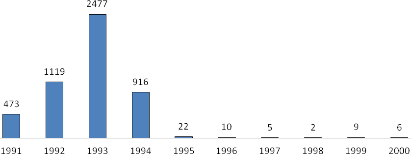 | Figure 1. Yearly inflation (%) in Brazil according to the Consumer Price Index (IPCA) from 1991 to 2000 |
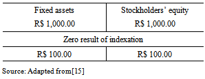
With respect to the impact of not recognizing the effects of inflation on Brazilian accounting, renowned researchers of Brazilian accounting strongly criticized the failure to consider the inflationary effects of the accounting statements prepared according to corporate legislation in force at the time. They studied the relevance of accounting information at “historic cost” and “constant currency” with data obtained from the Economática® database on listed Brazilian companies from 1996 to 2007. Their results pointed to the relevance of accounting information only for accounting practices at “historic cost”. To show the effect of indexation on fixed assets (FA) and stockholders’ equity (SE), the tables below show three situations demonstrating this method. For these examples we used an inflation rate of 10% applied on the figures shown. In situation 1, the FA and SE have the same value, so the net effect is zero, because they cancel each other; in situation 2, the SE is greater, so the net effect is a loss of indexation; in situation 3, the value of the FA is greater than that of SE, so there is a net gain from indexation, which is subject to income tax.Situation 1: The inflation index of 10% applied to the value of R$1, 000.00 of both the permanent assets and stockholders’ equity implies a gain and loss of R$100.00, meaning the net effect of indexation is a wash.Table 1. Nil Effect from Indexation on Fixed Assets and Stockholders’ Equity
 |
| |
|
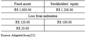
Situation 2: Here the value of the permanent assets is R$ 1,000.00 and of the stockholders’ equity is R$ 1,200.00, implying a gain of R$ 100.00 and a loss of R$120. 00, or a net loss of indexation of R$ 20.00.Table 2. Negative Effect (Loss) from Indexation on Fixed Assets and Stockholders’ Equity
 |
| |
|
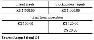
Situation 3: Here the value of the permanent assets is R$1,200.00 and of stockholders’ equity is R$ 1,000.00, implying a loss of R$ 100.00 and a gain of R$120.00, for a net gain of R$ 20.00.Table 3. Positive Effect (Gain) from Indexation on Fixed Assets and Stockholders’ Equity
 |
| |
|
The example presented by these three situations clarifies in a simple fashion how the decision on the capital structure, specifically between debt and equity capital, causes a range of possible effects of indexation on firms’ taxable income.
2.3. Fixed Assets
The increase in the fixed assets due to indexation was considered “monetary restatement revenue”, and the increase in stockholders’ equity was considered an expense. The question addressed here is whether before the advent of Law 9,249/95, Brazilian firms tended to have lower fixed assets and then after the end of indexation they increased their fixed investments. Due to the function of fixed assets in firms’ capital structure and the influence of indexation on the nominal value of these assets, several works have compared the makeup of Brazilian firms’ balance sheets with and without indexation. Of particular interest in these works is the inflationary gain on the tax liability and the effect of information in this respect in the capital market.In[16], it is investigated whether a variation in fixed assets caused a change in market expectations before and after the Real Plan. They found the variation in permanent assets to be a costly signal of investment decisions, that the capital market may react according to the firm’s signals as well as the country’s economic environment, and that the market became more efficient after the Real Plan. The results also indicated that firms, managers and shareholders should determine the correct moment to seek new funding for investments based on the share price, using debt when the stock price is low and issuing new shares when the price increases.
2.4. Debt
The option to increase the fixed assets is intimately related to the decision on financing between debt and equity capital. In this paper we examine the behavior of fixed assets and debt in two very different scenarios: a period of high inflation with indexation and taxation of the inflationary gain and a period of relatively stable inflation and no indexation. Various studies have been published on firms’ capital structure decisions, both in Brazil and internationally. Various studies have been published on the effect of inflation on firms’ capital structure decisions, both in Brazil and internationally”[7].In Brazil, it was analyzed the relationship between firms’ capital structure and variables representing intangible assets, such as the number of patents, average remaining validity period of patents and number of trademarks. The results indicated the absence of the influence of patents on the debt level of the firms analyzed. In another study, it was investigated the factors determining the choice on sources of funding of publicly traded nonfinancial companies in Brazil. Out of 356 listed firms, they analyzed a sample of 40. The results indicated that 13% of the firms consider opportunism, 50% adopt a capital structure target (static tradeoff), 28% follow the pecking order theory and 23% consider transaction costs as the most important factor in the decision on the capital structure.In an international perspective, in[8] it was studied the effects of inflation on the capital structure: the “Schal effect”, “Miller effect” and “DeAngelo-Masulis effect”. Regarding the first, the authors reported that an increase in firms’ aggregate debt is caused by the greater return on corporate bonds in relation to stocks as inflation increases. The second operates through the higher returns triggered by inflation on corporate bonds, which are taxable, in comparison with municipal bonds, which are not taxable. The third effect causes a reduction in the level of aggregate debt due to the increased tax deductible depreciation triggered by higher inflation. According to the authors, when lenders and borrowers enter into a loan agreement stipulating nominal values according to expected inflation and the real interest rate, the envisioned real interest rate changes when inflation changes unexpectedly, causing a transfer of wealth between debtors and creditors[2].Using the above three effects and added one more, called the Dammon effect, in[16] it was evaluated the effect of inflation on financial leverage. The results were not conclusive: he found that the capital structure is not subject to the dominant effect of any of these four factors.According to[11] that evaluated the level of debt, taxes and company value. He concluded that decisions on capital structure are irrelevant, because the firm value in equilibrium is independent of its capital structure, even when the interest paid is fully tax deductible.
2.5. Hypotheses
To assess the behavior of debt and fixed assets of the companies listed on the Bovespa between 1991 and 2000, we formulated two hypotheses. We believe that in the second interval, between 1996 and 2000 (period without indexation), companies acquired more fixed assets and incurred more debt in comparison to the first interval, covering the period from 1991 to 1995, (with indexation), and therefore presented higher levels of debt and fixed assets in comparison with the first group. The hypotheses are the following:H1: The period without indexation differs from the period with indexation with respect to firms’ debt and fixed assets.
3. Methodology
In this article we evaluated the average annual level of fixed assets and debt of firms listed on the Bovespa before (1991-1995) and after (1996-2000) the extinction of indexation in Brazil. For this purpose, we selected the firms with available data on total assets, fixed assets and indebtedness and calculated the ratios of fixed assets and debts per sector and applied analytical methods adequate for each sector. To assess the immediate effect of the extinction of indexation on the behavior of these ratios we made a year-by-year comparison of small groups.
3.1. Data Utilized
This study is empirical nature. We obtained the figures on the total assets, fixed assets and debt from in the balance sheets of 175 firms in the Economática® database, among the 656 companies listed on the São Paulo Stock Exchange (Bovespa). Of the 18 sectors into which these firms are divided, we considered the four most important, according to the number of firms, and used them in the sectoral analysis. All told there were 1,722 observations (balance sheets) in the database for the period from 1991 to 2000. The data on gross domestic product (GDP), a benchmark interest rate (SELIC) and exchange rate with the dollar (EXCHRATE) were obtained from IPEADATA.
3.2. Organization and Description of the Methods and Techniques of Criteria
a) Economic criterion:To analyze the behavior of fixed assets and debt in the periods with and without indexation, we used two techniques, analyzing the form of the relationship between the variables and comparing the means between the two groups. To study the relationship between the variables, we used the macroeconomic indicators gross domestic product (GDP), the basic interest rate (SELIC) and the exchange rate (EXCHRATE) because these satisfy the postulates of economic theory, namely they adequately describe and explain the variables of interest here, fixed assets and debt. These are indicators of economic growth, market interest rates and the dynamic of the external market. Based on economic theory, we also defined a priori the sign of the parameters. We assumed by definition that the model is a simplified representation of reality. It was structured to permit understanding the partial functioning of the firms in the periods with and without indexation, i.e., only what is relevant to the study, ignoring other aspects[10].b) Statistical criterion We treated the data to remove the effects of atypical or inconsistent values (outliers). Of the 656 companies listed on the Bovespa during the overall period, we eliminated financial institutions and those that were inactive or had zero ratios of fixed assets or debt in more than three consecutive years. We grouped the firms by sector within each period (the first from 1991 to 1995 and the second from 1996 to 2000). We only considered firms in existence in all the years of the period studied. We assumed in advance that the data come from a population with a normal distribution. To summarize and analyze the data we used Stata®, Excel and the Statistical Analysis System – SAS[19].To analyze the degree of relationship between the explanatory variables we used Pearson’s linear correlation. To test the hypotheses on this degree of relationship of the variables, we employed the correlation coefficient (r), with the probability of significance (p-value) along with the hypothesis that the true correlation of the population in question was zero.To explain the form of the relationship of the variables we used multiple linear regression analysis, in which the relationship was expressed in the form of a classic mathematical model. The evaluation statistics were obtained by analysis of variance, with the coefficient of determination (R2) to test the model fit, the F-statistic to test the significance of the joint effect of the explanatory variables on the dependent variable, and the Student-t statistic to test the significance of the estimated parameters or the hypothesis that a particular parameter was equal to zero. In all analyses, we considered a significance level of 5%.To evaluate the impact of the end of indexation on the behavior of the companies, we first tested two classic linear regression models: the first regarding the impact based on the ratio of fixed to total assets (FXASS_TA) and the second the ratio of debt to total assets (DEBT_TA). In both cases the explanatory variables were GDP, SELIC, EXCHRATE and a dummy for indexation (D_INDEX) to define the period before and after the end of indexation. Model 1: Fixed assets over total assets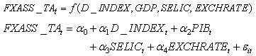 Model 2: Debt over total assets
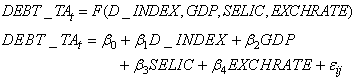 Where:● t: time interval of the analysis, 1991 to 2000;● β0: intercept;● β1 to β5: angular coefficient of each explanatory variable in the model;● FXASS_TA: ratio of fixed assets to total assets, calculated based on the balance sheets of the 175 firms analyzed in time t.● DEBT_TA: ratio of debt to total assets, calculated based on the balance sheets of the 175 firms analyzed in time t.Explanatory variables used:● D_INDEX: dummy variable for analysis of the periods before and after the end of indexation, where 0 represents the period with indexation and 1 indicates no indexation;● GDP: percentage variability of growth of gross domestic product;● SELIC: percentage variation of the average nominal basic interest rate;● EXCHRATE: variable expressed as an index of the exchange rate, with base 100 in 2005, which represents the variation of the average exchange rate (R$/US$).To complement the study of the form of the relationship and to support the hypothesis that the two periods were distinct, we employed a second test, the T-test. We used a multiple linear model to evaluate the behavior of the debt and fixed assets in the four groups of companies (by sector). For this test, we assumed that the two data sets were from distributions with the same variances. In calculating the variances and the linear correlation we used the SAS statistical package. In this package, the Proc Test routine performs a hypothesis test to check if the means of two populations are equal. We calculated a T-statistic for the test assuming that the variances were equal for the two groups, and another assuming the variances were different. To test the equality of the variances, we calculated an F-statistic. For each of the T- and F-statistics we associated the respective degrees of freedom and probabilities of significance (p-value). c) Econometric criterionTo check for the presence of multicollinearity, we used the Farrar-Glauber test[10]. The X2 statistic to carry out this test has a chi-squared distribution with[k(k-1)]/2 degrees of freedom. This was calculated in Excel according to the following formula:X2 = -[n – 1 – (1/6 *(2 k+5))] * ln det AWhere:n= sample sizek= number of explanatory variablesln= natural logarithmdet = determinant of the following matrix
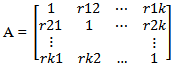 rij = simple linear correlation coefficient between Xi and XjFinally, we used the Durbin-Watson test[10] to check for the presence of serial autocorrelation or time dependence of successive values of the residuals, that is, whether the residuals are mutually correlated.
4. Results and Discussion
4.1. Description of the Data
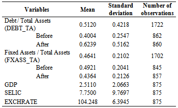
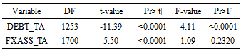
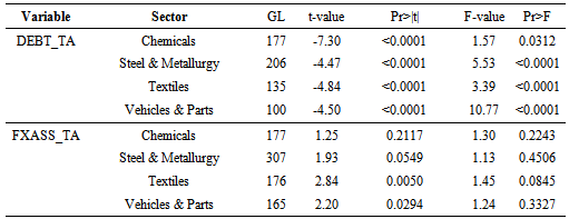
Table 4 presents the descriptive statistics of the variables of interest. The mean debt ratio (DEBT_TA) in the period before the end of indexation (DEBT_TA = 0.4004) is lower than in the period afterward (DEBT_TA = 0.6239). The contrary occurs for the fixed asset index (FXASS_TA), which declined from 0.4921 to 0.4364. In both cases, the data are more dispersed in the second period. These results indicate that firms changed their behavior in these respects with the end of indexation.Table 5 compares the means of the two periods both for DEBT_TA and FXASS_TA. According to the test of equality of the variances, the variances are not significantly different only for the fixed assets/total assets variable (F = 1.09 p-value = 0.2320), at the 5% significance. At this level there are significant differences between the means of the two periods for both DEBT_TA and FXASS_TA.Table 4. Descriptive Statistics of the Variables before and after the End of Indexation
 |
| |
|
Table 5. Analysis of the Periods with and without Indexation
 |
| |
|
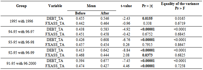
These results of the t-test suggest that the end of indexation influenced the level of fixed assets and debt of the firms. This indicates acceptance of the hypothesis that firms presented different levels of fixed assets and debt before and after the end of indexation.Table 7 presents the results of analyzing the immediate effect of the end of indexation, showing that in all years it increased, corroborating the hypothesis. Regarding the level of fixed assets, in the two last groups (1992-1995 to 1996-1999 and 1991-1995 to 1996-2000) there was a statistically significant decline, arguing against the hypothesis formulated. However, in the first two groups (1995 with 1996 and 1994/1995 with 1996/1997), although not statistically significant, the means increased according to the hypothesis, from 0.442 to 0.464 and from 0.451 to 0.458 respectively. Table 6. T-Test of Equality of the Means before and after Indexation, by Groups of Years
 |
| |
|
4.2. Multiple Linear Model
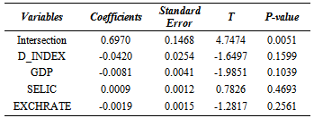
a) For the fixed assets/total assets ratio we obtained the following linear model:According to the F-test (F = 4.5198; P-value = 0.0646), H0 is rejected at the 5% significance. At the 10% significance level, the coefficients together are statistically different from zero. The value of R2 is 0.7833, meaning that 78.3% of the total variation of the fixed assets/total assets ratio is explained by the variables D_INDEX, GDP, SELIC and EXCHRATE. By the t-test, except for the intersection, all the others are significant at 5% (Table 7).Table 7. Fixed Asset Parameters Estimated
 |
| |
|
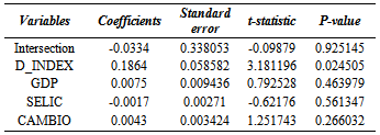
The dummy variable D_INDEX represents the sectional analysis of indexation, seeking to capture the temporal effect. The coefficient of -0.0420 indicates that in the period without indexation, the ratio of fixed to total assets declined, which runs counter to expected variation of this variable. However, this effect was not significant (p-value = 0.1599).With respect to the strength of the multicollinearity, the Farrar-Glauber statistic shows that for 10 degrees of freedom and 5% significance, the table value is Xc2=18.31. Therefore, since Xc2 is greater than the X2 calculated (X2= 6,622), the null hypothesis of the absence of multicollinearity is accepted at the 5% significance. Unlike the result of the T-test, this confirms the importance of the explanatory variables included in the model’s equation.The table of critical values of the Durbin-Watson statistic (d) for 5% significance, four explanatory variables and n = 10 provides a lower limit of dl = 0.376 and upper limit of du = 2,214. Since the d calculated by the model, dc = 1.8805, is between these two limits, d falls in the inconclusive region, that is, the hypothesis of the absence of serial autocorrelation can neither be accepted nor rejected. This is an outcome possibly caused by the sample size. Since d = 1.8805 is near 2, we choose to accept the hypothesis of no serial autocorrelation. This result also confirms the good specification of the mathematical form and that no important explanatory variable was omitted.b) Regarding the debt/total assets ratio, we determined the following model:The F-test (F = 9.5938; p-value = 0.0145) demonstrates that the coefficients, as a set, are statistically different from zero at the 5% significance. The R2 value is 0.8847, meaning that 88.5% of the total variance of the debt/total assets ratio is explained by the variables D_INDEX, GDP, SELIC e EXCHRATE.According to the T-test, except for the parameter of D_INDEX, all the others are significant at 5% (Table 8).Table 8. Estimated Indebtedness Parameters
 |
| |
|
As in the previous model, other factors could have influenced this non-significance of the majority of the explanatory variables. The possible causes were not detected by the methods used in the calculations of either multicollinearity or serial autocorrelation. Nevertheless, based on the non-significance of the explanatory variables, we believe it may be a problem of multicollinearity.The table of critical values of the Durbin-Watson statistic (d) for 5% significance, four explanatory variables and n = 10 provides a lower limit of dl = 0.376 and upper limit of du = 2,214. Again, since the d calculated by the model, dc = 1.8919, is between these two limits, d falls in the inconclusive region, that is, the hypothesis of the absence of serial autocorrelation can neither be accepted nor rejected. This is an outcome possibly caused by the sample size. Since d = 1.8919 is near 2, we choose to accept the hypothesis of no serial autocorrelation.The positive coefficient of D_INDEX (0.1864) demonstrates that in the period after the end of indexation the average debt over net assets increased in the proportion, confirming the expected direction of this effect. Unlike in the case of fixed assets/net assets, the period with indexation, indicated by this dummy variable, had a significant effect (p-value = 0.0245) of firms’ debt levels (Table 9).The signs of GDP and EXCHRATE are as expected, confirming that these variables have explanatory power over DEBT_TA. This direct relationship suggests that a strong economy has a positive effect on firms’ investments and productive capacity. The positive sign of EXCHRATE indicates that the debt grows when the Real is weaker. Since the majority of the firms in the sample export a good deal of their output, this behavior was expected. On the other hand, the negative sign of SELIC demonstrates that higher inflation tends to cause the ratio to fall, because the greater economic uncertainty that comes with higher inflation discourages investments. In summary, the model reflects what was expected with respect to the dependent variable.
4.3. Sectorial Analysis
4.3.1. Sectorial Analysis of the Estimated Parameters
With respect to the specific analysis of the equality of the means during the periods with and without indexation for sectors, of the four most representative chosen for analysis (Chemicals, Steel & Metallurgy, Textiles and Vehicles & Parts), the end of indexation did not influence the level of fixed assets/net assets in the Chemicals and Steel & Metallurgy but did in the other two, at the 5 % significance (Table 9).Table 9. Analysis of the Periods with and without Indexation by Sector
 |
| |
|
4.3.2. Multiple Linear Model by Sector
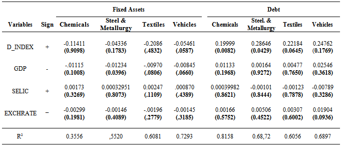
The analysis of the result for the four groups of companies shows that in all four sectors the level of debt increased after the end of indexation, while the level of fixed assets declined (Table 10). This behavior confirms the results obtained from the general model.Table 10. Estimated Parameters of Fixed Assets and Debt by Sector
 |
| |
|
As in the general analysis, the dummy variable D_INDEX represents the sectional analysis of indexation, seeking to capture the temporal effect. In Table 10 it can be seen that this variable, both for fixed assets and debt, presented the same behavior as in the general model. For fixed assets, the coefficients of -0.11411, -0.04336, -0.02086 and -0.05461 for the Chemicals, Steel & Metallurgy, Textiles and Vehicles sectors, respectively, indicate that in the period after the end of indexation, the ratio of fixed over total assets declined in these proportions, which runs counter to the intuitive expectation for the variation of this variable. Furthermore D_INDEX is only significant for the Vehicles sector, and then only at 10%. Regarding debt, the coefficients of 0.19999, 0.28646, 0.22184 and 0.24762 of this variable for the same sectors indicate that in the period after indexation, the ratio of debt to total assets increased in these proportions. In this case, the result agrees with the expected direction of variation of this variable. But here, unlike for fixed assets, D_INDEX is only not significant at 10% for Vehicles.Finally, except for the Chemicals sector, where the model for fixed assets presented R2 = 0.3556, the other values show that more than 50% of the total variation of the ratios fixed assets/total assets and debt/total assets are explained by D_INDEX, GDP, SELIC and EXCHRATE.
5. Conclusions
In this article, we are dealing with an issue very important as regards the investment and financing decision, namely the influence of taxation and the end of indexation in Brazil. The aim of this study was to assess the behavior of the levels of fixed assets and debt of Brazilian firms in relation to indexation for inflation. There are many studies in the international literature on the influence of inflation on accounting information, firms’ capital structure decisions and the effects of taxation in high-inflation settings.The results of this study indicate that the firms’ level of indebtedness increased with the end of indexation, while the level of fixed assets declined. Regarding the immediate effect, the level of debt in all the situations (1, 2, 3, 4 and 5 years) increased, as expected, while the level of fixed assets decreased in the five years after the end of indexation in relation to the five years beforehand, but increased in the comparison of one, to and three years before and after. This demonstrates that just after the end of indexation in Brazil, firms increased both their levels of fixed assets and debt.With respect to the key question of this study – whether the levels of fixed assets and debt differ in periods with and without indexation – the results indicate that both levels were different on average between the two periods. In relation to the analysis of the periods with and without indexation by sector (Chemicals, Steel & Metallurgy, Textiles and Vehicles & Parts), the absence of indexation only did not have an influence, at the 5 % significance, on the level of fixed assets/total assets in the Chemicals and Steel & Metallurgy sectors. The ratio of debt to total assets increased in all four sectors after the end of indexation, while the ratio of fixed to total assets declined, confirming the results of the general analysis.In sum the firms’ debt increased with the extinction of indexation, while the level of fixed assets declined. Important to emphasize that these results were the same when the firms were divided into the four main economic sectors. With respect to the key issue of this study, whether the level of fixed assets and debt differs in periods with and without indexation, the results indicate the existence of significant differences. This work contributes to show how tax rules, by impacting accounting information, influence the operational decisions of firms. The historical context of high inflation in Brazil offers a propitious setting to document the effects of the extinction of a tax accounting rule on corporate decisions regarding the levels of fixed assets and debt.This study does not exhaust the range of questions on the theme, and was limited to some extent in the choice of variables and the selection, collection and treatment of the data, with effects on the formulation of the models applied. Future studies could add other variables or refine the estimated parameters, as well as add information on the tax liability reported by firms to enable making inferences about the influence of tax considerations on corporate decisions. We hope this work has made a contribution to the study of indexation and call attention to the importance of the theme of the effect of taxes on business decisions.
References
| [1] | AARON, H. Inflation and the income tax. The American Economic Review, v. 66, pp. 193-199, 1976. |
| [2] | CLOYD, C.B.; LIMBERG, S.; ROBINSON, J. The impact of federal taxes on the use of debt by closely held corporations. National Tax Journal, Washington, v.50. no. 2, pp. 261-277, 1997. |
| [3] | Dreßler, D, The Impact of Corporate Taxes on Investment - An Explanatory Empirical Analysis for Interested Practitioners 2012. ZEW - Centre for European Economic Research Discussion Paper No. 12-040. Available at SSRN: http://ssrn.com/abstract=2105624. |
| [4] | Feld, L P.; Heckemeyer, J.; Overesch, M., Capital Structure Choice and Company Taxation: A Meta-Study, March , 2011. ZEW-Centre for European Economic Research Discussion Paper No. 11-075. Available at SSRN: http://ssrn. com/ abstract=1987613 |
| [5] | GROPP, R. E. Local taxes and capital structure choice. International Tax and Public Finance, Boston, v. 9. pp. 51-71, 2002. |
| [6] | HANLON, M.; HEITZMAN, S. A review of tax research. Journal of Accounting and Economics, v. 50. pp. 127-178, 2010. |
| [7] | HOCHMAN, S.; PALMON, O. The impact of inflation on the aggregate debt-asset ratio. Journal of Finance, v. 40. n. 4, pp. 1115-1125, 1985. |
| [8] | KIM, M. K.; WU, C. Effects on inflation on capital structure. The Financial Review, v. 23, p. 183-200. 1988. |
| [9] | LOPES. A.B.; WALKER, M., Asset revaluations, future firm performance and firm-level corporate governance arrangement: New evidence from Brazil. The British Accounting Review, v. 4, Issue 2, June 2012. p. 53 – 67. |
| [10] | MATOS, O. C. .Introduction to Econometrics: Theory and Application 3rd ed. São Paulo: Atlas, 2000. |
| [11] | MILLER, M. Debt and taxes. Journal of Finance, v. 32, pp. 261-257, 1977. |
| [12] | MILTO, F. Monetary correction: In essays on inflation and indexation. Washington, D.C.: American Enterprise Institute, 1974. |
| [13] | MORAES, R. C. Brazilian case and Hyperinflation, Porto Alegre, v. 21, n. 4, pp. 145-152, 1994. |
| [14] | MYERS, S. C. The capital structure puzzle. The Journal of Finance, v. 39, pp. 28-30. 1984. |
| [15] | NEVES, S.; VICECONTI, P. E. V. Advanced Accounting and Financial Analysis. 13th ed. São Paulo: Frase Editora, 2004. |
| [16] | NOGUERA, J. Inflation and Capital Structure. Working paper, n. 180. Nov. 2001. Available at: . Consulted on: 15 May 2011. |
| [17] | PANTEGHINI, P. M. Taxation, inflation, and the effective marginal tax rate on capital in Canada, Journal of Public Economic Theory, Volume 14, Number 1, 1 February 2012, pp. 161-186 (26). |
| [18] | PRINCEN, S. , Taxes Do Affect Corporate Financing Decisions: The Case of Belgian ACE. January , 2012. CESifo Working Paper Series No. 3713. Available at SSRN: http://ssrn.com/abstract=1992330. |
| [19] | SAS INSTITUTE. SAS User’s Guide: statistics. 5th ed. Cary (NC): SAS, 1982. p. 95. |
| [20] | SCHOLES, M.S. et al. Taxes and Business Strategy: A planning approach. 3rd ed. Upper Saddle River: Prentice Hall, 2004. |
 Abstract
 Reference
 Full-Text PDF
 Full-text HTML