1. Introduction

Over the last couple of decades, volatility has become one of the significant issues in the energy market. It is apparent that energy prices are the most volatile among all the commodity prices¹. Crude oil, coal, natural gas and other oil related products all observe significant price fluctuations. These fluctuations in prices create uncertainty in the minds of consumers and producers. Reference[2] and[15] assert that investors and market participants delay investment because of this uncertainty. Again, this delay in investment results in inefficient resource allocation in the long-run. Persistence in volatility and the asymmetric effect of volatility are two crucial aspects of the volatility modelling. Generally, volatility increases in response to positive and negative shocks. However, this increase in volatility is not in equal magnitude to the same level of positive or negative shocks. This characteristic of volatility is captured by asymmetry. For energy return volatility, asymmetry is observed in opposite direction. Energy returns volatility reacts more to positive shocks than to negative shocks, suggesting volatility of energy return increases more when energy price increases than when energy price decreases. Like other financial and economic series, energy price returns also exhibit persistence in volatility. Persistence implies that any shocks to conditional variance endure. The return series tend to follow a pattern, i.e. large changes are followed by large changes and small changes are followed by small changes². Volatility persistence has significant impact on derivatives in where underlying is energy prices. Reference[16] mentions the price of options and other derivative varies if the volatility of that underlying commodity is persistent. In the literature of energy price volatility, most of the studies aim to find out the best model for forecasting volatility accurately. Moreover, most of the studies deal with crude oil whereas natural gas and coal also play significant role in the energy market. To the best of our knowledge, this paper is the first of its kind which considers both asymmetry and persistence of major three energy price volatilities after controlling Global Financial Crisis (GFC). Comprehensive understanding of asymmetry and persistence is imperative in correctly estimating volatility of energy prices, forecasting future energy price volatility and understanding of the broader financial markets and the overall economy.

The main objective of this paper is to model the volatility of various energy returns and compare the asymmetry and persistence aspect of these energy returns volatility. In this case, we estimate the volatility of three main energy components of crude oil, natural gas, and coal. For volatility modelling of energy returns, we use conditional volatility measures. For conditional measure of volatility we apply various extensions of ARCH and GARCH models. We employ threshold GARCH (TGARCH) for evaluating volatility asymmetry and fractionally integrated GARCH (FIGARCH) for measuring persistence. We also aim to evaluate the effect of GFC on the return and volatility of energy prices. This GFC leads to sharp decline in demand for output and therefore, the demand for commodity also declines. This results in plummeting commodity prices. It is hypothesised that this current GFC brings structural shift in volatility of commodity prices. In this study, we use dummy variable for GFC and evaluate the effect of GFC on return and volatility of energy prices.

The construction of the paper is as follows: Section 2 discusses recent and related studies; Section 3 discusses about our models for this study; Section 4 deals with the data and its descriptive statistics; Section 5 shows the estimated results, and finally, Section 6 concludes the study.

2. Literature Review

Asymmetry aspect in volatility is initially observed in stock return volatility by reference[3] and[6]. In stock market, negative shocks lead to higher volatility than positive shocks. In case of commodity and energy returns, asymmetry is observed in opposite direction. Energy return volatility reacts more to positive shocks than to negative shocks. For studying asymmetry in crude oil volatility, Reference[14] uses exponential GARCH model to evaluate varying effects of positive and negative shocks on oil return volatility. Reference[5] also studies the asymmetry effect on two crude oil prices: WTI and Brent crude oil. He finds that volatility reacts more to negative shocks than to positive shocks. However, it is evident only for Brent crude not for WTI crude oil. The literature on asymmetry of energy prices is limited to crude oil prices.

Persistence or long memory plays a crucial role in volatility forecasting and it has immense influence in risk management, derivative pricing and portfolio management. Persistence implies that any shocks to volatility do not die quickly rather its effect endures. Among the studies, [12],[16],[20] and[21] examine persistence in oil return volatility. Reference[16] estimates volatility persistence of crude oil and natural gas using GARCH and ‘half-life’ volatility measure and finds the evidence of persistence in the volatility of crude oil and natural gas. However, his measure of persistence suggests that the fluctuations are short-lived than previously assumed. If there is a shock to crude oil or natural gas prices, it lasts up to 5 to 10 weeks. Reference[20] estimates volatility persistence for larger number of energy commodities including crude oil, gasoline, heating, natural gas, and propane. In a recent study, Reference[19] estimate persistence in crude oil and find the evidence of long memory even with structural break.

3. Methodology

To facilitate our study, we use TGARCH and FIGARCH- two extensions of GARCH class model. Constant variance or homoskedasticity in the error term is common assumption; however,[10] and others identify that the assumption of constant variance in the error term is not valid and require a flexible model to describe the volatility in the data. The researchers observe conditional variance or heteroskedasticity in the error term. GARCH model can capture this heteroskedasticity in the error term. Moreover, the GARCH model can accommodate persistence and asymmetry in volatility. The GARCH (p, q) is modelled by[4], and this model allows current conditional variance to depend on p- past conditional variances and q- past squared error terms. GARCH models are well established in volatility modelling considering various attributes of volatility. Reference[1],[12],[13] and[16] use various GARCH models for their study of energy return volatility. Reference[18] uses various parametric and non-parametric volatility models for commodity prices and finds that GARCH and its variants fit better over other modeling techniques. Reference[22] contends that univariate models like TGARCH and FIGARCH perform better when asymmetry in volatility is considered.

For both TGARCH and FIGARCH, we consider the same mean equation; however, the specification of conditional variance will be according to the structure of the model. Both mean and variance equation of the models include dummy variable GFC. The mean equation is as follows:

(1)

where, is the energy price return at time t, GFC is the dummy variable for financial crisis in 2008, t-bill is the 3 month US Treasury bill rate, and is the error term in the mean equation at time t. Since carrying cost is one of the important components of the return function of energy commodity prices, we use carrying cost in the return function of energy price returns. In this case, we use T-bill to represent the carrying cost. Reference[16] states that the risk free rate is a significant component of this carrying cost and it can be used to represent the carrying cost. Reference[16] also uses 3 month U.S. Treasury bill rate in his study of crude oil and natural gas return volatility. The mean and variance equation are augmented by dummy variable GFC³ to identify the shift in volatility in energy prices due to the recent financial crisis. In the variance equation, the ARCH and GARCH parameters must be positive, α>0, and β>0, and the sum of quantifies the persistence of shocks to volatility. As the return series is unexpectedly large in either the upward or downward direction, the GARCH specification captures the volatility clustering effect.

3.1. Threshold GARCH (TGARCH)

(2)

where I_t-1 =1 if <0; =0 otherwise.

For asymmetric effect, we would see . The condition of non-negativity is, , , and . In equation (2), measures constant volatility, measures the effect of lagged return shocks of energy on its volatility and measures the effect of the previous period’s conditional volatility on the volatility of current period. The term captures the asymmetry effect of energy return volatility. If there is a symmetric effect of lagged shocks on the volatility is zero. In contrast, if lagged negative shocks augment the volatility by more than lagged positive shocks , there is an asymmetric effect which is typically associated with a leverage effect or a volatility feedback effect. If lagged negative shocks decrease the volatility of energy returns the asymmetric effect typically found for equity is inverted, i.e. positive shocks of energy return increase its volatility by more than negative shocks. For energy returns, the expectation is that positive shocks have more effect on volatility than negative shocks. Therefore, we expect negative sign in .

3.2. Fractionally Integrated GARCH (FIGARCH)

In general GARCH class models, the stationary ARMA process is a short memory process and the autocorrelations are geometrically bounded. In this case, autocorrelation decreases rapidly. However, researchers observe that some time series exhibit large degree of persistence. To accommodate this persistence in autocorrelations,

The FIGARCH (1, d, 1) model takes the following form:

(3)

where, , , , ; is the fractional integration parameter and L is the lag operator. The parameter characterizes the persistence property of hyperbolic decay in volatility because it allows autocorrelations to decay at a slow hyperbolic rate. The advantage of the FIGARCH process is that for , it is sufficiently flexible to allow for intermediate ranges of persistence. The FIGARCH model allows for long memory behaviour and a slow rate of decay after volatility shocks.

4. Data

This study includes daily closing prices of crude oil, coal, and natural gas. For crude oil, natural gas, and coal we use 2-month future price⁴ of West Texas Intermediaries (WTI), Henry Hub and ICE Global Newcastle futures price respectively. All the data sets have 3912 daily observations covering the period of 1 January 1995 to 31 December 2012. All the data are collected from Datastream. We use continuously compounded energy price return- natural logarithm of the ending price less its natural logarithm of the beginning price.

The descriptive statistics for the return series of energy prices of crude oil, natural gas, and coal are summarized in Table 1. The average returns of energy prices are positive. The annualized returns of energy prices vary from 2.5% for natural gas to 10% for coal. For crude oil, average annualised return ranges from 5% to 7.5%. In case of standard deviation, all the variables have less than 2% except natural gas with standard deviation of 4%. The energy price returns also exhibit skewness and kurtosis. The crude oil and natural gas price returns are skewed to left and coal price returns are skewed to right. In case of kurtosis, all the variables show the evidence of leptokurtosis, as the values of kurtosis are greater than three. Considering skewness and kurtosis, none of the variables of this study is normally distributed. The thick tails of excess skewness can be modeled by assuming a conditional normal distribution for returns. Again, this normality is tested using Jarque-Bera (J-B) test. The probability values of J-B test indicate that the null hypothesis is rejected which implies the variables are not normally distributed. For modelling purpose, we also check the presence of unit-root and ARCH effect in the data⁵. The ADF and PP test of unit root results show that the first difference of prices series is free from the presence of unit root as we reject the null hypothesis of the presence of unit root. LM test confirms that the return series exhibits the presence of ARCH effect.

Table 1. Descriptive statistics for daily energy price return

5. Results and Discussion

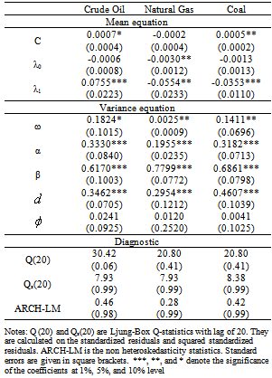
The estimation results of TGARCH and FIGARCH are presented in Table 2 and 3. The mean equation is same for both models and they take a constant term, T-bill rate and dummy variable for GFC. For crude oil forward price, the results of the mean equation show that the coefficient of constant, , is statistically significant. However, it is not statistically significant for coal and natural gas. The coefficient of the constant is negligible. The coefficient of T-bill, , is statistically significant for all energy price returns except in TGARCH model for natural gas. This result is consistent with theory, as the return of energy prices is a function of carrying cost. In our model, T-bill rate is a proxy measure of carrying cost of energy prices. The coefficient of t-bill rate has positive coefficient suggesting when t-bill rate goes up, the returns energy returns also go up. Reference[16] also has the same results for T-bill rate in the mean equation. We have important findings for the effect of recent global financial crisis. Although the coefficients of dummy variable GFC is not statistically significant in the return function of the energy prices, GFC has effect on the volatility of energy price returns suggesting GFC contributes to the energy return volatility. The results of the variance equation show that the coefficients of the dummy variable GFC, , are significant for all energy prices and for all GARCH class of models. In most of the cases, the coefficients of GFC are significant at 1% and at 5% level.

Table 2. FIGARCH estimation results for crude oil, gas and coal

5.1. Persistence in Volatility

One of the main objectives of this paper is to measure and compare the persistence of volatility of different energy returns. In the variance equation of (3), the GARCH term, , captures persistence of shocks. When the coefficient, , is close to 1, the shocks to volatility do not die out quickly. To measure the persistence of shocks, we estimate FIGACH (1, d, 1) model using equation (3). In the model, when fraction term is , the volatility has long memory and underlying series is stationary and when , the volatility does not have long memory. Our estimated results from Table 2 show that the coefficients of are statistically significant and its value ranges from 0.2954 (gas) to 0.4607 (coal). The results imply that the volatility of energy returns exhibit long memory and any shocks to the volatility do not die out quickly. The results are confirmed by the coefficient value of . The value of is less than unity. Wei et al. (2010) also find the evidence of long memory in two types of oil returns. Using FIGACRH model, they estimate persistence of Brent and WTI oil return volatility and their coefficients value range from 0.310 to 0.443. For measuring volatility persistence in energy return volatility, we also discuss about half-life, another measure persistence of volatility.

The ‘half-life’ is another measure of volatility persistence. Reference[8] defines half-life as the time required for the volatility to move half way back towards its unconditional mean. The unconditional mean of the FIGARCH (1, 1) model is estimated as the ratio of the constant term (ω) in variance equation to the difference between 1 and the sum of ARCH and GARCH terms. Reference[16] measures half-life using the following equation:

(4)

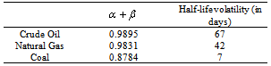
Table 3 shows the estimates of persistence of energy returns using and half-life volatility measure. The second column of Table 3 contains the sum of and from the estimation results of equation (3) and the third column contains half-life measure of volatility. The estimation identifies that the returns volatility of energy returns exhibit long memory, since the sum of and is always less than one⁶. Among the energy prices, coal has strong mean reversion. It means that the volatility of coal approaches their average or long-run volatility relatively quickly. On the other hand, other energy prices volatility has also mean reversion; however, their volatility is relatively persistent, since the sum of and is close to one.

Table 3. Half-Life volatility measures of crude oil, gas, and coal

The half-life measure of volatility of energy prices indicate the same phenomenon described using the sum of and and mean reversion. As coal is relatively less persistent and its volatility moves quickly to their long-run volatility level, the half-live for coal is also relatively less. This result implies that shocks to the volatility are very transient. Crude oil return volatility exhibits the highest level of persistence. The half-life of crude oil is 67 days. It implies that any shocks to this volatility take 67 days to return half-way back without any further shocks to that volatility. On the other hand, the half life volatility of natural gas is 42 days suggesting that any shock to natural gas takes 42 days to return half way back to its volatility.

5.2. Asymmetric Effect of Volatility

To examine the existence of asymmetry in the volatility of crude oil, natural gas, and coal, we estimate TGARCH (1, 1) model by using equation (2). The asymmetry is measured by the sign and the significance of the coefficient. Our estimated results show that asymmetry is evident in the volatility of crude oil and gas whereas the same is not evident in case of coal.

The results of the TGARCH model estimation confirm the existence of asymmetric effect on the volatility of energy returns of crude oil, natural gas. The coefficients of ARCH and GARCH terms, , and , are statistically significant. It ensures that the lagged residuals and lagged conditional variance are significant in describing the conditional volatility. The sign of is negative TGARCH model suggesting the positive shocks have higher impact on next period conditional volatility of energy return than negative shocks. This result is consistent with our expectation of positive energy price shocks have higher effect on volatility than negative price shocks. The coefficient estimates vary from -0.0029 for coal to -0.0212 for crude oil. The coefficients of asymmetry are relatively higher in oil suggesting that when energy price increases, oil return volatility is affected relatively higher than other energy commodities.

Table 4. TGARCH estimation results for crude oil, gas and coal

For robustness check of our estimated models, we employ Ljung-Box Q-statistics for autocorrelation, and LM test for checking the presence of ARCH effect in the residuals. The Q statistics for residuals evaluates the misspecification of mean equation of the GARCH models and Q statistics for squared residuals evaluate the misspecification of the variance equation of our models. We select 20 lags. Our result shows that both the mean and variance equations are correctly specified and no correlation is evident in the residuals of our models. The calculated result of ARCH LM test in the residuals shows that ARCH effect is not present in the residuals, since the null hypothesis of the tests cannot be rejected Based on Q-statistics and ARCH LM, all our GARCH models estimated in this paper is adequately specified and well fit.

6. Conclusions

In this paper, we measure the volatility of crude oil, natural gas, and coal, and evaluate the persistence and asymmetric aspect of their volatility. We use TGARCH and FIGARCH modelling technique for capturing asymmetry and persistence respectively. We also employ half-life volatility measure. Our estimated results from half-life volatility measure state that coal exhibits strong mean reversion implying shocks are not persistent in their volatility. On the other hand, shocks in crude oil volatility are very persistent. For future price of crude oil, shocks last for 67 days and for spot price of crude oil, shocks last for 48 days. Natural gas has also relatively higher level of volatility persistence. TGARCH model is used to evaluate asymmetric aspect of volatility of the energy series. It is expected that volatility increases more by positive shocks than by negative shocks. The asymmetry coefficient is relatively higher for crude oil. In terms of evaluating asymmetric aspect of volatility, our estimation suggests that except coal return volatility, asymmetry is observed in the volatility of crude oil, natural gas.

This research is of great importance to risk managers, port folio managers, policy makers, and market participants to understand volatility of major energy components. Energy derivative market is one of the largest derivative markets and efficient pricing of such derivatives requires accurate estimation and understanding of volatility. Our focus is on asymmetry and persistence of volatility to understand nature of energy volatility precisely.

Notes

1. Reference[9] calculates that oil has 78% and natural gas has 38% annual price volatilities. Reference[17] calculates volatilities of different commodities and finds that crude oil prices are 65% more volatile than other commodities.

2. Reference[13] notes that large changes tend to be followed by large changes, of both sign, and small changes tend to be followed by small changes.

3. GFC is dummy variable and it is constructed using Eviews add-in ‘Create US recession dummies’.

4. In Datastream, the longest available future price for crude oil is 2-month future price.

5. The results of unit root test and ARCH effect are not shown due to space constraint. The results can be available upon request.

6. We check the significance of sum of α and β. In null hypothesis the sum of α and β is equal to one or greater than one. The hypothesis tests imply that for all energy prices we reject the null hypothesis. Therefore, the volatility measures are persistent in their nature. The hypothesis test results are not reported.