-
Paper Information
- Next Paper
- Previous Paper
- Paper Submission
-
Journal Information
- About This Journal
- Editorial Board
- Current Issue
- Archive
- Author Guidelines
- Contact Us
International Journal of Finance and Accounting
p-ISSN: 2168-4812 e-ISSN: 2168-4820
2013; 2(7): 348-364
doi:10.5923/j.ijfa.20130207.03
Does the History of Ex-ante Abnormal Earnings Growth Forecasts Affect Earnings Response Coefficient
 Abstract
 Reference
 Full-Text PDF
 Full-text HTML
1Department of Accounting and Finance, School of Business Administration, Oakland University, Rochester, MI 48309, USA
2Department of Accounting, Economics, Finance, and Management Information Systems, The School of Business Administration and Economics, The College at Brockport, State University of New York, Brockport, NY 14420, USA
Correspondence to: Yin Yu, Department of Accounting and Finance, School of Business Administration, Oakland University, Rochester, MI 48309, USA.
| Email: |  |
Copyright © 2012 Scientific & Academic Publishing. All Rights Reserved.
After the economic recession in 2008, the U.S. business community became more concerned about earnings quality. This paper applies the earnings response coefficient (ERC) methodology and the abnormal earnings growth (AEG) model to examine whether firms with consecutive positive abnormal earnings growth in previous years exhibit a higher ERC than other firms. We then use this approach to detect whether these firms report high quality earnings. Accounting research has focused on ERC to investigate the usefulness of accounting earnings in explaining stock returns. Extant research on valuation theory has shown that AEG drives firm value. Our results support the hypothesis that annual returns are higher for firms with consistent positive abnormal earnings growth forecastsinferred from analysts in a consecutive three-year rolling window. For these firms, we furthershow that post earnings announcement analyst forecast revisionsin the following year are more pronounced. We also find that the forecast revisions are even more pronounced when the history of positive/negative abnormal earnings forecasts are consistent with the sign of positive/negative forecast error in current year. The finding also indicates that analysts tend to place less weight on positive current year earnings surprise if firms show three-year negative abnormal earnings forecast in current and prior two year. From valuation analysis perspective, we document that equity premium are higher for firms which not only meet or beat analyst expectations but also have a history of positive AEG forecasts than firms without such a history.
Keywords: Earnings Response Coefficient, Abnormal Earnings Growth, Permanent Earnings
Cite this paper: Yin Yu, Yuanlong He, Does the History of Ex-ante Abnormal Earnings Growth Forecasts Affect Earnings Response Coefficient, International Journal of Finance and Accounting , Vol. 2 No. 7, 2013, pp. 348-364. doi: 10.5923/j.ijfa.20130207.03.
Article Outline
1. Introduction
- This study explores the effects of concurrent unexpected earnings with a history of sustained abnormal earnings growth (AEG, hereafter) forecasts implied from analysts on the quality of earnings and earnings response coefficient (ERC, hereafter). This study demonstrates that firms with a history of sustained positive AEG have higher ERCs applied onto their contemporaneous unexpected earnings thanfirms without such a history. Reference[1] is the first study to document a positive relation between earnings and stock returns. The authors used past earnings as an anchor for their unexpected earnings specification. Additional literature indicates that analyst forecast is a better proxy for use in the unexpected earnings specification. Subsequently, an abundantliteraturedocuments evidence consistent with the use of past earnings, zero earnings and analyst forecasts as thresholds that firms would like to meet or exceed, albeit with different intensity[2, 3, 4], and perhaps with earnings and/or expectation management [5].Reference[6] shows that firms with a pattern of increasing earnings have higher ERCsthan those without such a pattern. However, there are two possibilities for firms with similar patterns of increasing earnings: earnings either increase at a rate lower than firms’ cost of capital or at a rate greater than their cost of capital1. For those firms withearnings increases but negative abnormal earnings growthin the current year, their cum-dividend earnings growth rate is lower than their cost of capital. Recent developments in valuation theory make two important observations about earnings. First, there is a “savings bank” of earnings associated with any expectation of next period earnings. This suggests that earnings should grow at least at the rate of cost of capital.Second, dividends, when paid out, create a wealth effect that reduces future earnings. Abnormal earnings growth, therefore, is the net effect of these two forces. Further, the valuation framework outlined by reference[7] suggeststhat abnormal earnings growth can serve as an earnings benchmark. If future earnings continuously grow over and beyond the cost of capital, then earnings create value. AEG also suggests that any new value-relevant information about earnings must be incorporated into information about abnormal growth. From this perspective, using merely past earnings as an anchor to measure sustained growth in multiple periods would be tantamount to functional fixation on earnings.In this study, we empirically test whether the market takes into consideration sustained ex-ante abnormal earnings growth pattern when valuing the firm.We find that the market does reward firms with a history of sustained positive AEG by assigning higher value multipliers to these firms.Our empirical test is conducted bypartitioning firms into three groups:the first includes firms with sustained favorable AEG inferred from analysts; the second group comprises firms with sustained unfavorable AEG; and the third contains firms with mixed AEG in a consecutive three-year rolling window. Next we test the return earnings association for these three groups after controlling for contemporaneous earnings news (or unexpected earnings). As implied from the valuation theory, wealsoexamine the effect of sustained favorable/unfavorable AEG forecastson predicting future operating performance. Previous literature suggests that persistence of earnings, accrual quality and earnings volatility are the most frequently used measures of earnings quality[8]. In our analysis, we rely on ex-ante AEG forecasts to distinguish earnings quality. We find evidence suggesting that earnings innovation in the current year is more likely to be permanent andrelevant for those firms with a history of sustained favorable AEG. These firms are highly likely to show promising future prospects than firms without such a pattern.Previous literature also documents other signalsin addition to earnings for distinguishing high versus poor earnings quality, such as sustained revenue-supported growth in earnings and meeting-or-beating revenue forecasts[9,10]. In this study, we consider abnormal earnings forecasts asa leading indicator of future performance and valuation. We predict that firms with a sustained favorable AEG forecast will be more likely to meet or beat three earnings thresholds: reporting an earnings increase, reporting a profit,or meeting or beating analyst expectations. We find that firms are more likely to report a profit and/or an increase in earnings, but we find no evidence of an association between a firm’s AEG forecast history and meeting-or-beating analyst expectations (MBE, hereafter). Evidence in the accounting and finance literature shows that the market pays close attention to unexpected earnings and responds to the magnitude of forecast error[5,11]. Studies have identified a distinctive valuation premium/ discount to the act of meeting-or-missing analyst forecasts even after controlling for the magnitude of forecast error[12]. If both sustained ex-ante AEG forecasts and MBE are indicators of firms’ performance, then we predict that ERC will be more pronounced if MBE in the current yearconfirms firms’ positive or negative AEG forecasts over the previous three years.The regression result supports our prediction that the market more strongly rewards thosefirms that meet-or-beat analyst forecastsin the current year and also have sustained AEG forecasts in the past. The market penalizes firms that both miss analyst forecastbenchmarksandhave consecutive negative abnormal earnings forecasts inferred from analysts over the past three years.This paper contributes to the literature by associating AEG forecastswith the earnings response coefficient. We empirically confirm that AEG forecasts play an important role in firms’ valuation using theOhlson and Juettner - Nauroth valuation framework. This study extends previous work by showing thatthe market considers firms’ earnings surprise to be of “true superior performance”when using abnormal earnings growth as the valuation anchor. The remainder of the paper is organized as follows. Section 2 discusses the relevant literature and our hypothesis development. Section 3 describes the methodology. Section 4providesour sample selection and descriptive statistics. Section 5 presents the empirical results, and final section offers concluding remarks.
2. Background Literature and Hypothesis Development
2.1. A Review of the Abnormal Earnings Growth Model[7] as a Valuation Framework
- The abnormal earnings growth model (AEG) decomposes firm value into (a) capitalized next period earnings and (b) capitalized future abnormal earnings, which is the most important determinant of value. The AEG model presented in (1) also serves as a theoretical background for exploring and testing the relations among the future earnings growth rate (long-term and short-term), the PE ratio and the cost of capital.
 | (1) |
 is the capitalized forward earnings in the subsequent period.
  equals 1 plus
  , and
, and  is the firm’s cost of capital. Subscript tdenotes the time period.
  is abnormal earnings, defined as
  ;
;  is the dividend paid out at time t. In the above equation, the time-series distribution of
  follows an assumption:
 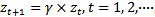 , where
  (
( , where
 ) is the long growth parameter.Reference[13] shows that γ is a measure capturing both asymptotic growth in earnings and asymptotic growth in the future dividend payout growth ratio.This model anchors on next period expected earnings and adopts the earnings perspective that earnings add value in the future, which allows the model to handle multi-stage growth of earnings per share. An appealing earnings property is imbedded in the model: earnings dynamics (ED)[14]. The following ED equationis derived from the Hicksian definition of earnings and is based on the condition of no arbitrage:2
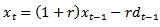 | (2) |
 , which translates into fundamental value discounted by the cost of capital. More intuitively, positive abnormal earnings growth implies earnings are growing beyond the cost of capital. Substituting the notation
  with
with  , the formula becomes
 | (3) |
 is the earnings per share in period t-1. Substituting realized earnings
  with analyst forecast
  , we get the abnormal earnings growth forecast implied in analyst forecasts:
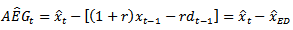 | (4) |
 formula, analyst forecast of earnings becomes two components of forecasts.
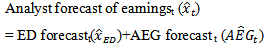 | (5) |
2.2. ERC Literature and Hypothesis Development
- Early seminal work[1] associates stock price with the earnings surprise from earnings announcements and provides the evidence that earnings is useful in investor decision making. Many additional earlier studies apply the same methodology that associates security return with unexpected earnings to demonstrate that unexpected earnings is used as a primary input and explanatory variable in equity valuation models. References[15, 16, 17] document a positive association between earnings persistence and ERCs, indicating more persistent earnings have a stronger stock price response. Therefore, an increase in persistence will lead to positive equity returns. Reference[18] also documents a positive association between ERCs and growth. A proper benchmark of persistent and permanent earnings should reflect underlying firm performance and measure sustainable future cash flows that will be discounted to reflect firms’ value. Reference[8] summarizes earnings quality proxies across literature. The following measures have been used: earnings persistence, abnormal accruals (accrual quality), earnings smoothness, asymmetric timely loss recognition and target beating. References[19, 20] suggest that greater fundamental uncertainty about a firm’s future cash flows will cause a larger stock price reaction. In addition, such fundamental uncertainty about future cash flows is highly associated with uncertainty in earnings. Because ERC represents the overall quality of earnings, our primary objective in this study is to show that ERC is affected by fundamental AEG expectationsinferred from analysts in Ohlson and Juettner-Nauroth’s valuation framework. We anticipate a higher equity market valuation of concurrent earnings innovation if analysts consistently anticipated a positive AEG in the past years. Reference[21] documents that when earnings do not follow a random-walk model, earnings change is not a good predictor of market value and does not serve as a good proxy for earnings expectation. Following the argument in[21], we contend that the response of the AEG forecast over time rather than the lagged earnings change should be considered a permanent earnings shock. We expect a lower correlation between transitory earnings and contemporaneous stock returns according to reference[21]. Reference[22] finds that firms with relativelyhigherex - ante uncertainty in earnings, as measured by analyst forecast variance, tend to have smaller and less significant ERCs. Reference[6] finds that the market rewards those firms if they exhibit patterns of increasing earnings in multiple consecutive years. The pattern of earnings increase is related to economic determinants of risk and growth. Continuously increasing earnings reflects growth over time. However, the authorsdo not distinguish among the alternative sources of growth in earnings. Sustained increases in earnings can be achieved through different components in earnings. Reference[9] documentsthat firms with sustained earnings increases supported by revenue growth have higher ERCs, higher future performance and less earnings management. As the AEG model shows, a largerAEG persistence will lead to a higher ERC. Thus, we predict the following hypothesis:H1: An ex-ante AEG forecast has a systematic effect on the market response to unexpected earnings. In multiple time periods, firms will have higher ERCs if they have sustained positive ex-ante abnormal earnings growthexpectationsinferred from analyst.An AEG forecast is a separate and credible signal of firms’ future performance since it is modeled into the valuation framework and associated with superior growth ability in earnings beyond the cost of capital. Accordingly, we test our second hypothesis:H2: In multiple time periods, firms with a pattern of continuously favorable AEG forecastswill exhibit higher future performance in the following period. If firms have sustained ex-ante AEG forecasts from analyst, it is highly likelythese firm will deliver favorable earnings news, as measured by alternative thresholds documented in the literature (reporting a profit, reporting an earnings increase or meeting/beating analyst expectation). An equity premium from benchmark beating is documented in other studies[5, 6, 12]. If AEG is the leading valuation input, then we hypothesizethe following:H3: In multiple time periods, firms with a pattern of continuously favorable AEG forecasts in the past three year are more likely to exceed other earnings thresholds in the subsequent period. Analysts constantly update their forecasts upon receiving new information about corporate earnings. Forecast revisions are widely used for investment decisions inthe investment community. Reference[22] provides evidence on upward and downward revisionsthat were perceived as good and bad news by the market. If analysts’ forecasts incorporate abnormal growth expectations into their revised forecasts, then we would expect the following:H4: Analyst forecasts revisions will be more pronounced for firms that have a pattern of positive ex-ante AEG forecasts in the past. Reference[10] tests the assumption that multiple signals such as earnings and revenue signals are more credible for firms delivering superior performance. Theauthorsdocument that the ERC to MBE is even pronounced when revenue forecastsare also met. MBE is perceived by the market as either good news or bad news, depending on whether the market expectation is missed. The OJ valuation framework models AEG forecasts as both value creation and value destruction measures. Combining two signals gives us our final hypothesis: H5: IfAEG forecasts in multiple periodsindicate consistent value creation of firms’ earnings, then ERCs will be more pronounced if those firms also meet or beat analyst forecasted expectations in the current year.
3. Methodology and Research Design
3.1. Abnormal Earnings Growth Forecast Measurement
- Figure 1 provides a timeline of earning series events, including earnings announcements, analyst forecasts of earnings, abnormal earnings growth forecasts and measurement points for the variables. Returns are measured contemporaneously with earnings periods. The return is 12-month market risk-adjusted return. The return window encompasses 8 months prior to and 4 months after the earnings announcement for year t-1 earnings. Analyst forecast revision is the difference between
 and
and  . Consecutive abnormal earnings growth in the past three yearsis defined as
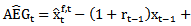
 ; and
; and  , respectively. We use IBES actual earnings to maintain comparability with analyst forecasts of earnings. The variables are defined as follows:t= the time subscript (year 1988, 1989, ….. or 2009);
 = the first analyst forecast for year t made in year t afterthe t-1 earnings announcement;
 = the last analyst forecast for year t made in year t-1 before the t-1 earnings announcement;
 = the first analyst forecast for year t-1 made in year t-1 after the t-2 earnings announcement;
 = the first analyst forecast for year t-2 made in year t-2 after the t-3 earnings announcement;
 and
and  = the estimated cost of capital for year t-1, t-2 and t-3, respectively, calculated by the methodology developed in reference[23];
 and
and  = the announced annual earnings for year t-1, t-2 and t-3, respectively, obtained from IBES;
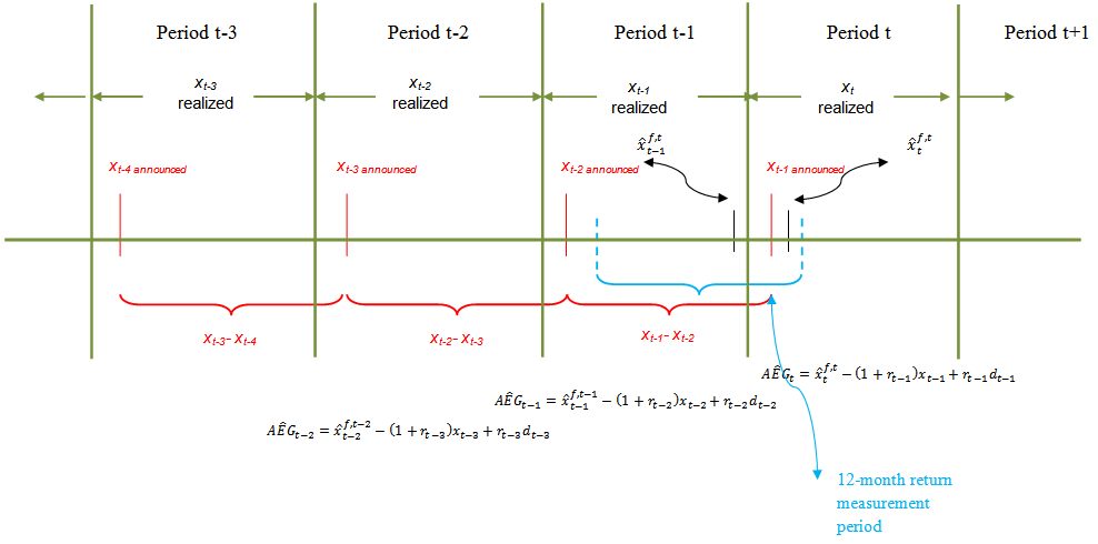 | Figure 1. Timeline of Return, Earnings Announcement, Forecast and Abnormal Earnings Forecasts |
 and
and  = annual dividend calculated by partially compounding the quarterly dividend by considering the quarterly time factor (1.75, 1.5, 1.25 and 1). Calculating AEG for each year requires the prior year’s dividend amount. The dividend is paid quarterly throughout the year, meaning that investors have several more months use ofthe first three quarters’ dividends than of the amount distributed in later quarter. To account for this effect, we use partially compounded dividend for reinvested dividend in ED’s calculation.
3.2. Cost of Capital Estimation
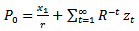
- We estimate firm-specific cost of capital and long term growth parameter γusing a portfolio approach developed by[23]. This method assumes that 20 firms grouped into the same portfolio based on their PEG4 ratios have the same cost of capital and the same gamma. The estimation equation from[23] is as follows: ceps2 / P0 = α + β * eps1 / P0, where α = r *(r – γ), β =1 + γ, and ceps25 is the forecast of two-period-ahead cum-dividend earnings, which is ceps2 =ceps2+rdps1.
3.3. Regression Analysis
- We use the following model to test our prediction that ex-ante AEG has a systematic effect on the market response to unexpected earnings.

 RET(-8, +4) is the cumulative abnormal return based on the marketrisk-adjusted model for the return window (eight months before the annual earnings announcement date and four months after the announcement date).6 FEis the unexpected earnings, which is the difference between actual announced earnings
  and the mean consensus analyst forecast, scaled by the beginning year stock price. DAEG_3+ (DAEG_3-) is a dummy variable that takes a value of 1 if abnormal earnings forecasts are continuously positive (negative) in the past three year:
  ,
,  and
and 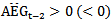 .First, we estimate ERC by separating firms into two groups: those whose expected abnormal earnings growth is consistently positive in the three-year rolling window and all other firms. Further, we expand model 1a by separating firms into three groups: those whose expected abnormal earnings are positive in the three-year window, those whose are negative, and all other firms. The predicted signs of
  and
and  are positive, positive and negative, respectively. The following models are used to examine whether the analyst forecast revision incorporates past abnormal earnings forecast about future earnings growth.
 REV is the analyst forecast revision, which is the difference between analyst forecast earnings for year t after and before the year t-1 earnings announcement
 .We allow different levels of persistence on profits and losses because losses are less persistent and tend to be more transitory[24]. Reference[12]shows that analysts weigh positive forecast error more heavily than negative error. We separate forecasts into
  and
and  . Both REV and FE are scaled by stock price at the beginning of the year.
  is a dummy variable representing the number of yearsthat AEG is positiveover the past three years. For example,
  equals 1 if AEG in any two years in a three-year window is greater than 0, and zero otherwise.
  is equal to 1 if AEG in any one year in a three-year window is positive, and 0 otherwise.
  is a dummy variable equals 1 if ex-ante abnormal earnings growth is positive in at least one of the past three-year rolling window, and 0 otherwise. We use the following models to test whether the market assigns a higher ERC when a firm delivers three-year value creation signals consistent with meeting-or-beating analyst expectations in the current year.
 MBE (MISS) is an indicator variable equal to one if the announced earnings for t-1 are greater than or equal to(less than) the consensus analyst forecast made in year t-1. All other variables are defined as aforementioned. We estimate Model 3a by partitioning firms into two groups: those with positive AEG in all years in the three-year window and all other firms.Model3b is estimated based on positive or negative AEG in each of the years in the three-year window and all other firms. In Model3b, when the ex-ante AEG forecast in the past three years confirms with MBE (MISS) in the current year, ERCs are a combination of the coefficients
  . When they are inconsistent with each other, ERCs are the coefficient combinations of
  and
and  represent the case when ex-ante AEG is positive in at least one year out of the three-year window and MEET or MISS analyst expectation in current year. We predict that the coefficient combinations of
  and
and  have the most significantly positive and negative magnitudes, respectively.
 3.4. Accounting Measure for Future Performance
- Future performance is estimated at the end of year t after estimating
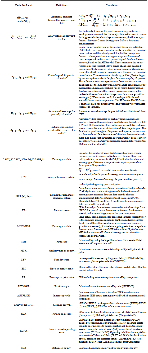
 in the three-year rolling window. We use the following accounting performance measures to test the prediction that positive abnormal earnings growth forecast in the past three years will lead to higher future profitability: return on net operating assets (RNOA), return on assets (ROA), return on equity (ROE), sales growth (∆REVN/ REVNt-1), income growth (∆NI/PRICEt-1), and profit margin (PFTMGN). Since FASB statement No. 115, the appreciation of financial assets and liabilities has been close to market value. The model developed by[25] assumes financial assetsare already valued, but operating activities are not yet valued and contribute to the value premium beyond the current book value. The authors also find that RNOA is not the only driver for residual income; the other driver is growth in net operating assets. RNOA is calculated as operating income after depreciation (Compustat OIADP) divided by beginning net operating assets (NOA). We use beginning NOA as the ratio denominator to isolate the impact of the contemporaneous growth effect in NOA. Net operating assets are calculated as operating assets less operating liabilities. Following[26]7, operating assets are calculated as total assets (Compustat AT) less cash and short-term investments (Compustat CHE) and investments and other advances (Compustat IVAO). Operating liabilities are calculated as total assets (Compustat AT) less debt in current liabilities (Compustat DLC), long-term debt (Compustat DLTT), the book value of total common and preferred equity (Compustat items CEQ and PSTK), and minority interest (Compustat MIB). All variables are defined in the Appendix.
 4. Sample and Descriptive Statistics
4.1. Sample Selection
- The sample period is from 1988 to 2009 and only firms whose fiscal years end December 31st are chosen to ensure the cost of capital estimation in the same calendar year period for each portfolio. Following[23], we use the same method to simultaneously estimate the firms’ cost of capital and long-term change in the firms’ abnormal earnings growth rate (γ). The estimation of cost of capital requires the year-ending closing price, the dividend from Compustat,and earnings forecast either pulled directly from or calculated from IBES database. Our initial sample consists of all firms covered in IBES and Compustat, both active and inactive. The cost of capital estimation requires firms to have four or more years of earnings forecasts, earnings announcement dates, and quarterly dividend data with adequate financial statements data. For example, the estimation for firm year 1988 started from 1983 to ensure that the firm has adequate data to estimate the cost of capital using this procedure. These restrictions allow us to calculate AEG in three consecutive years. The procedure allows sustained growth but excludes extreme high growth and risky firms that may affect ERC[9]. After we calculate firms’ AEG in a consecutive three-year rolling window, we expand the window into a subsequent one year period, the realization period of year t. Thus, we also require that the firms have analyst forecasts and accounting data available for year t. Stock prices and returns from CRSP must be available as well. To mitigate the potential effect of outliers, we remove the top and bottom 1% of firm-year observations for analyst forecasts, stock prices, expected AEG, revenue and net income. Our final sample comprises 3,848 firm-year observations.
4.2. Descriptive Statistics
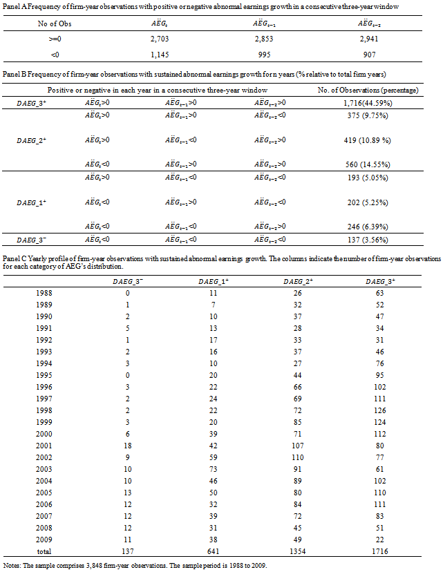
- Table 1 presents the distribution of firm years along with the number of years of sustained earnings growth based on our 3,848 observations. Panel A reports the number of firm years with positive/negative AEG in a three-year rolling window. Most of the firms have positive
 in one year of the three-year window. Positive
  firms decrease steadily from the first to the third year. Panel B presents the distribution of firm-year observations by sustained AEG across the three-year window. There are 1,716 (44.59%) and 137 (3.56%) firm years with positive or negative AEG, respectively, in all three years. There are 1,995 (51.88%) firm years with positive
  in either two or one years. Among those observations, 1,354 observations have positive
  in two years. Panel B also reports each combination of the signs for
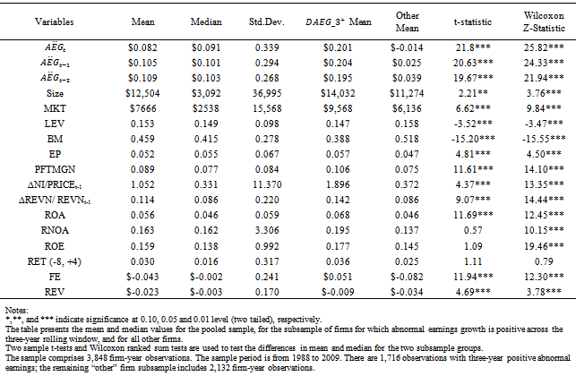
  (either positive or negative) in any single year of the three-year window. Panel C presents the time profile of the sample years, indicating the number of firm years in which AEG is positive within the three-year rolling window. It appears that firms with long strings of positive growth in abnormal earnings expectations are more prevalent in the period between 1997 and 2000 and between 2004 and 2006. This pattern seems to reach its peak in 1998 and starts to fall after that. The second downward trend starts in 2007.Table 2 presents the means and standard deviations of variables used in the test, plus some other variables that capture firm characteristics. Table 2 also presents the mean value of the main variables for the
  subgroup of firms and for all other firms, and shows two sample t-tests and Wilcoxon ranked sums tests for differences in means and medians, respectively, across the two subsamples. Table 2 reveals a pattern of higher accounting performance, lower leverage and large market capitalization being associated with sustained ex-ante AEG expectations in multiple years. Specifically,
  firms have significantly higher profit margin (0.106), change in NI (1.896), change in sales (0.142), RNOA (0.195), ROE (0.177). The table also reveals that
  firms have larger forecast errors (0.051), forecast revisions (-0.009), size (14.032), book-to-market ratios (0.388), earnings-to-price ratios (0.057) but smaller leverage ratios (0.147).
|
|

5. Test Results
5.1. ERC
- Table 3 presents regression statistics for Models 1a and 1b using yearly and pooled samples of firms from 1988 to 2009. The results from the pooled sample are not tabulated. Panel A of Table 3 reveals that for firms with consecutive positiveAEG expectations (
 ), the coefficient on α2(2.6479) is significantly positive. This finding indicates that the market assigns a larger ERC for these firms after controlling for analyst forecast error in the current period. The mean coefficients are reported with t-statisticsin parentheses, obtained using the Fama-MacBeth procedure of dividing the means of the annual coefficients by their standard errors. The Fama-MacBeth t-statistic of α2 in Model 1a is 2.14, statistically significantly at the 5 percent level. We further extend the model by separating firms into three groups by including two dummies (
 and
and  ).
).  is assigned a value of 1 if firms have negative AEG expectations in all three years. The coefficient on
  is significantly positive at the 5% level (
 =2.5037, Fama-MacBetht-statistic=2.01), indicating that there is an incremental valuation response on forecast error for those firms with positive AEG forecasts across the three-year window. However, for firms that have negative AEG expectations across the three-year window (
 ), the coefficient is not significant. These results suggest that investors only perceive consistent positiveAEG expectations to be more sustainable and value relevant.
 5.2. Future Performance
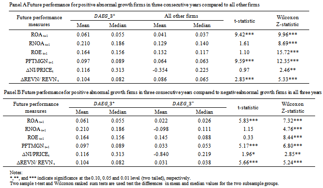
- Table 4 presents the results of future operating performance based onex-ante AEG expectations. Panel A provides the mean and median values of the performance measures for the
 subgroup and for all other firms.Panel B decomposes all other firms into two additional subgroups: negative AEG in all three years versus negative AEG in at least one year but not all three years. We choose negative AEG in all three years for testing purpose. The last two columns report the t-test and Wilcoxon Z test for the differences among these subgroups.In Panel A, the Wilcoxon ranked sums test shows that the median values of all operating performance measures are significantly higher for those firms with positive AEG than for all other firms. This result is consistent with the findings in reference[27] that AEG is associated with future accounting and stock performance. Two-sample t-tests only show significance in the differences for ROA, profit margin and sales growth. Our main interest is comparing firms with sustained positive AEG forecasts withfirms with negative forecasts in three years. Panel B shows that the differences in magnitude are even more pronounced between these two subgroups. The results confirm our prediction that poor future performance is more acute for firms with negative AEG forecasts in the past three years. The Wilcoxon ranked sums tests show that the differences among the median values remain statistically significant for all measures. Two sample t-tests show no difference in valuesin terms of subsequent year RNOA and ROE. Overall, the results in Table 4 are consistent with our prediction in H2 that ex-ante positive AEG indicates better future performance.
5.3. Other Earnings Thresholds
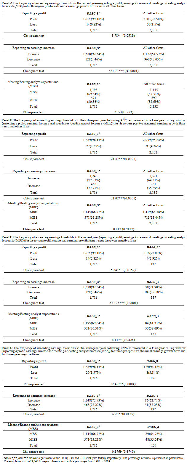
- Table 5 reports whether the frequency of reporting a profit, avoiding earnings decreases, and meeting-or-beating analyst expectationsare associated with an ex-ante AEG pattern. Panel A indicates whether the frequency of exceeding earnings thresholds in the current year would be much higher for three-year positive AEG firms than for all other firms. The current year refers to the last year in which ex-ante abnormal earnings growth forecasts were measured in a three-year rolling window. The results are tabulated in a 2x2 table by three thresholds and the type of firm. Results show that firms with positive ex-ante AEG expectationsacross a three-year window are more likely to report a profit (99.18%, χ2 =3.78, p<0.0519) and report an earnings increase (92.54%, χ2=661.70, p<0.0001), but that they are not more likely to beat analyst expectations (69.64%, χ2=2.39, p<0.1223).
|
|
|
5.4. Forecast Revisions
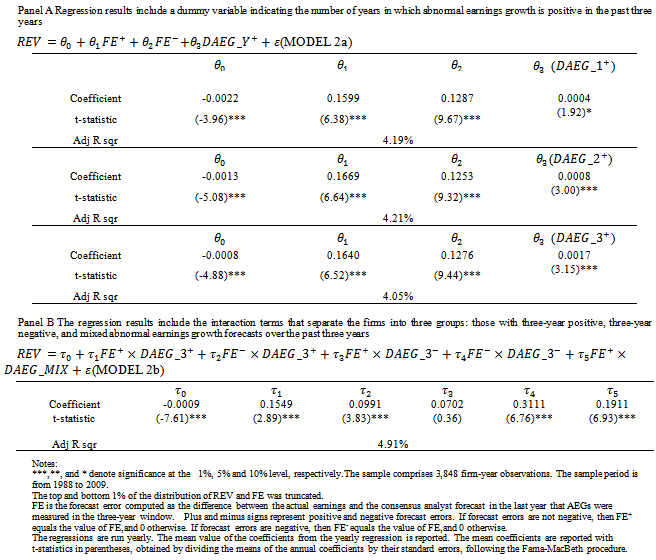
- Table 6 presents the regression results for Models 2a and 2b, which examine whether analysts incorporate prior year abnormal earnings forecast indicators into their revisions.8 The results for Model 2a show that the coefficients on the positive θ1 and negative θ2 forecast error are all statistically significant, indicating that analyst forecast revisions adjust upward and downward for positive and negative forecast error, respectively, accordingly to contemporaneous earnings innovations. For example, the coefficient on FE+(0.1669) when
 is included is significantly higher than the coefficient on FE- (0.1253), indicating that analysts weight positive forecast errors more heavily than negative errors in forming their conditional expectations for future earnings. This result is consistent with the findings in reference[12]. The coefficients on
  (0.008) and
  (0.0017) are significant at the 1% level, indicating that analyst forecasts, on average,revise their forecasts by incorporating the number of years in the past three years that firms had a positive AEG forecast. If firms only have one year with a positive AEG forecast
  ), analysts incorporate this information but it is only significant at the 10% level (t=1.92). Table 6 Panel B shows the estimation results for Model 2b in which we separate firms based on whether they have positive, negative or mixedex-ante AEGexpectationscontinuously across the three-year window. The coefficient on
  is 0.3111 (t-statistic=6.76, p-value<0.0001), showing that analysts assign a significant downward revision to firms that have a negative forecast error for year t-1 earnings and three straight years of negative AEG expectations. The coefficient on
  (0.0702)) is insignificantly positive, indicating analysts do not revise their forecasts upward for firms with a history of consistently negative AEG forecasts even though those firms deliver positive unexpected earnings in year t-1. Overall, the results show that analysts use AEG expectations when revising their forecastsof future earnings.
5.5. Valuation Consequences of AEG Forecasts along with MBE
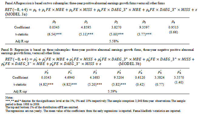
- Table 7 presents the regression results for Models 3a and 3b. The mean coefficients are reported with t-statistics in parentheses, obtained by dividing the means of the annual coefficients by their standard errors, following the Fama - MacBeth procedure. Table 7 Panel A presents the results for two subsamples: firms with positive AEG forecasts across the three-year window versus all other firms. If firms not only meet-or-beat expectations (MBE) but also have
 , the coefficients are │ρ1│+│ρ3│. If firms fail to MBE buthave three years of positive AEG forecasts, the coefficients are │ρ2│+│ρ4│. If firms only MBE(MISS) analyst expectations without having a sustained AEG pattern, the coefficient is │ρ1│(│ρ2│). Only ρ4 has an insignificant coefficient, indicating that when firms fail to MBE in year t-1, the market does not assign a higher value multiplier even though the firms have had three consecutive years of positive AEG forecasts in the past. Model 3b is based on separating firm observations into three-year positive, three-year negative, and mixed AEG forecasted across the three-year window. Consistent with our predication in H5, when AEG expectationsare consistent with MBE, the ERCs are more pronounced:
  equals 14.2192, which is statistically significantly higher than when firms have positive three-year AEG forecasts but fail to meet analyst expectation
  (4.7803). The difference is significant at the1% level (F-test is 14.04). The coefficients on
  are also significantly higher than
  (4.6940) at the 1% level (F-test=14.21). The coefficient on
 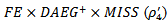 is 0.6120 which is insignificantly positive, indicating the market does not seriously punish firmsthat have a three-year history of positive AEG when they miss analyst forecast expectations. The coefficients for firms fail to MBE but have a positive AEG expectations in all three years are
  . The coefficients for firms thatmeet-or-beat analystexpectationsand have unstained AEG expectation are
  . The comparisons of coefficients are insignificantly different from each other. We summarize the analysis of ERCs for all combinationsin Table 8.When firms have mixed AEG forecasts in the prior three years, the market treats them no differently,regardless of whetherthey meet analyst expectations (
 vs
vs  ). Compared with firms that fail to meet-or-beat analyst expectations, the incremental effect of having consistent negative AEG forecasts is 3.5570 but it is not statistically significant at the 10 percent level. Even though these firms meet the analysts’ expectations, the market does not reward them significantly (
 =3.3824). For firms with sustained positive AEG forecasts, the market significantly rewards them if they also meet the analyst expectations (
 =9.5204). The market perceives this phenomenon as confirming signals.
|
|
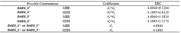
- The evidence partially confirms our prediction in H5 that the market assigns the most pronounced ERC to those firms, when firms meet analyst expectation with sustained positive AEG forecast pattern in prior period. However the market does not distinguish these firms with those meeting – or - beating the analyst expectations but having a history of consistently negative AEG forecasts. The evidence documented in prior literature suggests firms that meet or beat analyst expectations consistently have a distinct market premium in addition to their unexpected future earnings[12]. The reward to MBE is independent of firm performance[5]. Our results from Table 8 suggest that such a premium can be partially explained by the history of abnormal earnings growth expectationsinferred from analysts.
6. Concluding Remarks
- This research examines whether firms achieve a higher value multiplier (ERCs) by having a history of consistent positive abnormal earnings growth forecasts inferred from analysts in consecutive three years. We document that valuation consequences and post-announcement analyst forecast revisions are more pronounced for firms with positive AEG expectations inthree consecutive years, even after controlling for contemporaneous earnings forecast error. We also find that the forecast revisions are even more pronounced when the history of positive/negative abnormal earnings forecasts is consistent with the sign of positive/negative forecast error in the last year of the measurement window. These findings indicate that analysts place less weight on positive current-year earnings surprise if firms show three consecutive years of negative abnormal earnings forecasts. After controlling for unexpected earnings, analysts incorporate the sign of abnormal earnings growth history into their forecasts and revise future earnings accordingly.Moreover, we find that future earnings performance is higher for firms with a history of positive abnormal earnings growth forecasts than those without such a pattern. This predication is inferred based on the relation between abnormal earnings growth forecasts and a firm’s equity value under Ohlson and Juettner-Nauroth valuation framework. Our findings indicate that investors will anticipate higher future earnings for firms with a history of consistent positive abnormal earnings growth forecasts inferred from analysts. The higher value is beyond the contemporaneous period forecast error. We also find thatthese firms are more likely to report a profit and avoid earnings loss in that year and the following year. We show evidence that firms with such apattern is not associated with the possibilities of meeting-or-beating analyst expectations. Our findings therefore suggest that the firms without such a history of consistent positive abnormal earnings growth expectations may achieve MBE by other means. From the valuation analysis perspective, we further document that equity premium are higher for firms that not only meet or beat analyst expectations but also have a history of positive AEG forecasts compared to firms without such a history. The evidence also implies when firms fail to meet expectations but have one-year or two-year positive abnormal earnings growth forecastsover the previous three years, the market punishes them significantly; however the market does not differentiate these firms from those that have three straight years of positive AEG forecasts but fail to meet-or-beat expectations. This evidence may suggest that investors perceive firms with consistently positive abnormal earnings expectations as less risky. We find the market penalizes firmsthatboth miss analyst expectations and exhibit a consistent negative history of abnormal earnings forecasts; however, the incremental punishment is not significant when comparing to those firms with a mixed AEG forecast history. Our empirical evidence indicates that abnormal earnings growth should be considered a value-relevance factor for interpreting earnings implication. This study suffers from the following limitations. If we assume xt-1, xt-2 and xt-3 form the basis for forecasting xt, xt-1 and xt-2, then returns should be a function of
 and
and  . However, a better proxy for investors’ expectation of xt would probably be γxt-1, where γ is an expected earnings growth rate that takes dividend paid-out into account. Therefore, annual return surrounding year t-1, t-2 and t-3 earnings announcement are likely to be better explained by
 and
and  . Our proxy for γt-1xt-1 is
  , where “r” is the discount rate or normal growth rate, and we denote this r-based estimate of γt-1xt-1 as earnings dynamics-based forecast. In other words, our motivation is to determine if
  ,
,  and…form the basis for investor expectations for the subsequent year’s earnings. Investors should be forecasting earnings based on what they expect a firm can achieve rather than on “normal” earnings growth. For example, if last year’s ROE was 15%, this performance is expected to continue, and the firm pays no dividends, then we expect xt = xt-1 * 1.15 even if the cost of capital is 10%. Even though we use prior ROE as a substitute for r estimated by Easton method in the robustness check and we achieve similar results, we are not sure what role normal earnings growth (10% in this case) should play in investor expectations in this respect. Second, by using the Easton model, the paper becomes a joint test of the Easton model’s ability to measure ex-ante cost of capital and whether investors incorporate cost of capital into their earnings forecasts. Reference[28] document it may result in incorrect references about the magnitude of estimated coefficients and about the differences in coefficient behavior between groups of firms if the underline assumptions about the equality of firm-specific coefficients and equality of firm-specific unexpected earnings variance are rejected when using pooled cross-sectional regressions instead of using firm-specific models.. They find ERCs are much larger by using firm - specific coefficient methodology than by using cross - sectional regression approach. Firm observations in each year may be different due to our data restriction when calculating AEG forecast in the three-year rolling window. Therefore, their procedure[28] may not apply to our data. We use the pooled cross-sectional regressions for testing our hypotheses due to the availability of data;therefore our results may be biased in this regard. Reference[28] investigates short-term event study of ERC but our study focuses on the long-term association design.Based on U.S. empirical data, overall our results indicate the market pays attention to the earnings dynamics-based earnings forecasts to form earnings expectations as well as uses them to differentiate permanent from transitory earnings.
Appendix Variable Definition
Notes
- 1.
 , where G = the cum-dividend earnings growth rate; R= 1+r is the required rate of return or 1 plus the cost-of-equity capital; and
  and
and  are the earnings per share and dividend for year t-1, respectively. When firms have earnings increases but have negative AEG, then the formula transforms to
  .2.
.2.  and
and  then we have
  is the risk-free rate.3. This is because
  when
when  .4.
.4.  5. Following reference [23], a circularity problem incurs since calculating ceps2 requires the estimated cost of capital, yet ceps2 is used to estimate r. As in [23], we also assume the displacement of future earnings due to the payment of dividend is 12 percent. This is based on the assumption that if these dividends had been reinvested within the firm, they would have earned a return equal to the historic rate of market return. We also use an iterative procedure, starting from r equals to 12 percent and keep revising the estimates of r until there is no further change in the revised estimates of r and γ. 6. We estimate stock betas using the capital asset pricing model (CAPM). To estimate beta, we use monthly return extending from 48 months to 12 months prior to announcement dates. 7. In their study, growth in NOA has mean-reversion properties, and they show that growth in long-term NOA reduces future profitability.8. Untabulated results show that positive ex-ante AEG firms have a scaled analyst forecast revision that is 0.003% higher than for firms with consistently negative AEG forecasts across all three years. The difference is statistically significant (t test=2.56, p-value<0.02). The Wilcoxon sum ranked tests confirm that the difference inthe median value is statistically and significantly different, as well.
References
| [1] | Ball, R., & Brown, P. (1968). An empirical evaluation of accounting income numbers.Journal of Accounting Research, 6, 159-178. |
| [2] | Brown, L. D., &Caylor, M. L. (2005). A temporal analysis of quarterly earnings thresholds: propensities and valuation consequences. The Accounting Review, 80, 423-440. |
| [3] | Degeorge, F., Patel, J., &Zeckhauser, R. (1999). Earnings management to exceed thresholds.Journal of Business, 72, 1-33. |
| [4] | Burgstahler, D., &Dichev, I. (1997). Earnings management to avoid earnings decreases and losses.Journal of Accounting and Economics, 24, 99-126. |
| [5] | Bartov, E., D. Givoly, & C. Hayn. 2002. The rewards to meeting or beating earnings expectations. Journal of Accounting and Economics, 33, 173-204. |
| [6] | Barth, M.E., Elliott, J. A.,& Finn, M. W. (1999). Market rewards associated with patterns of increasing earnings. Journal of Accounting Research, 37, 387-413. |
| [7] | Ohlson, J.A., and Juettner-Nauroth, B.E. (2005). Expected EPS and EPS growth as determinants of value.Review Accounting Studies, 10, 349-365. |
| [8] | Dechow, P., Ge, W., &Schrand, C. (2010). Understanding earnings quality: A review of the proxies, their determinants and their consequences. Journal of Accounting and Economics 50, 344-401. |
| [9] | Ghosh, A., Gu, Z.,& Jain, P. C. (2005). Sustained Earnings and Revenue Growth, Earnings Quality, and Earnings Response Coefficients.Reviews of Accounting Studies 10: 33-57. |
| [10] | Rees, L., &Sivaramakrishnan, K. (2007). The effect of meeting or beating revenue forecasts on the association between quarterly returns and earnings forecast errors. Contemporary Accounting Research 24, 259-290. |
| [11] | [Lopez, T.J., & Rees, L. (2002). The effect of beating and missing analysts' forecasts in the information content of unexpected earnings.Journal of Accounting, Auditing & Finance, 17, 155-184. |
| [12] | Kasznik, R. &Mcnichols, M. F. (2002). Does meeting earnings expectations matter? Evidence from analyst forecast revisions and share prices. Journal of Accounting Research, 40, 727-759. |
| [13] | Ohlson, J., &Gao, Z. (2006). Earnings, Earnings Growth and Value.Foundations and Trends in Accounting, 1 (1), 1-70. |
| [14] | Ohlson, J.A. (1991). The theory of value and earnings and an introduction to the Ball-Brown analysis.Contemporary Accounting Research, 8, 1-19. |
| [15] | Kormendi, R., &Lipe, R. (1987). Earnings innovations, earnings persistence, and stock returns. Journal of Business, 60, 323-345. |
| [16] | Easton, P. D., &Zmijewski, M.E. (1989). Cross-sectional variation in the stock market response to accounting earnings announcements.Journal of Accounting and Economics 11, 117-141. |
| [17] | Collins, D.W., Kothari, S. P.,& Rayburn, J. D. (1987). Firm size and the information content of prices with respect to earnings. Journal of Accounting and Economics,9, 111-138. |
| [18] | Collins, D.W., & Kothari, S. P. (1989). An analysis of intertemporal and cross-sectional determinants of earnings response coefficients. Journal of Accounting and Economics, 11, 143-181. |
| [19] | Holthausen, R. W., and Verrecchia, R. E. (1988). The Effect of Sequential Information Releases on the Variance of Price Changes in an Intertemporal Multi-Asset Market. Journal of Accounting Research 26, 82-106. |
| [20] | Robichek, A.A., & Myers, S. C. (1966). Valuation of the firm: Effects of uncertainty in a market context. Journal of Finance, 21, 215-227. |
| [21] | Ali, A., &Zarowin, P. (1992). Permanent versus transitory components of annual earnings andestimation error in earnings response coefficients.Journal of Accounting and Economics, 15, 249-264. |
| [22] | Imhoff, E. A.,& Lobo, G. J. (1984). Information content of analysts’ composite forecast revisions.Journal of Accounting Research, 22, 541-554. |
| [23] | Easton, P. D. (2004). PE ratios, PEG ratios, and estimating the implied expected rate of return equity capital. The Accounting Review, 79, 73-95. |
| [24] | Hayn, C. (1995). The information content of losses.Journal of Accounting and Economics,20, 125-153. |
| [25] | Feltham, G., &Ohlson, J. (1995).Valuation and clean surplus accounting for operating and financial activities.Contemporary Accounting Research, 11, 689-731. |
| [26] | Nissim, D., &Penman, S. (2001). Ratio analysis and equity valuation: from research to practice. Review of Accounting Studies, 6, 109-54. |
| [27] | Yu, Y. (2010). Future earnings performance and stock value predictability of the expected abnormal earnings growth strategy. Working paper.Oakland University. |
| [28] | Teets, W., &Wasley, C. (1996). Estimating earnings response coefficients: pooled versus firm-specific models. Journal of Accounting and Economics, 21, 279-295. |