Yuriy V. Kozyr
Department of Theoretical Economy and Mathematic Research, Central Economics and Mathematics Institute of Russian Academy of Sciences, Moscow, 117418, Russia
Correspondence to: Yuriy V. Kozyr, Department of Theoretical Economy and Mathematic Research, Central Economics and Mathematics Institute of Russian Academy of Sciences, Moscow, 117418, Russia.
| Email: |  |
Copyright © 2012 Scientific & Academic Publishing. All Rights Reserved.
Abstract
This article considers the structure of interest rate, applied for discounting of risky cash flows. The purpose of the article is a presentation of ways of reflecting inflation and risks in the calculation of risk discount rate. In introduction on base of well-known dependences is shown that risk premium depends on inflation rate and (for multiplicative-type models) risk free rate. In the first part of the article three Interest rate algebras are presented. They describe the attitude between nominal discount rate, risk free rate, inflation rate and risk-premium. This algebras can presents in additive-type or multiplicative-type versions and have given risk premium value without detailed description the structure of risk premium. The second part of the paper has more detailed attitude between risk premium, risk free rate and mathematical expectation of losses because of bankruptcy/default. It is shown that the obtained dependences are slightly different and depends on the initial preconditions calculation: the principle of arbitration or the principle of certainly equivalent.
Keywords:
Interest Rate, Risk Free Rate, Risk Premium, Probability of Losses
Cite this paper: Yuriy V. Kozyr, The Interest Rate Algebra, International Journal of Finance and Accounting , Vol. 2 No. 4, 2013, pp. 220-224. doi: 10.5923/j.ijfa.20130204.05.
1. Introduction
There are many different interpretations for structure of interest rate: unbiased expectations theory, liquidity preference theory, liquidity premium. Also exist many different models for discount rate valuation, such as CAPM, MCAPM, APM and etc. However most of this models don’t give possibility of direct connection between such parameters as inflation, real rate and risk premium. This article contains a version of interest rate algebra sets developed by the author and applicable for the interpretation of structure for risk-free (in first part) and risky (in second part) interest rates. According to the established tradition, the analysis of the structure of interest rate for the purpose of its subsequent use in discounting exercises involves the following relations: Irving Fisher Expression [1]: | (1) |
where, r – nominal rate of interest,rr – real rate of interest,i – the rate of inflation for the period,Furthermore, decomposition of an interest rate into a risk-free component and the risk premium can be expressed as [2], [3], [4], [5]: | (2) |
where, r – the interest rate specific to future cash flows from a project (asset) with a certain investment risk, rf – interest rate on risk-free investments,pr – risk premium for bearing the risk of investing into similar projects (assets).Thus, the work of the classics of investment theory affords the conclusion that the level of interest rate is a function of the risk-free rate (net of inflation), the rate of inflation, and the risk premium component: | (3) |
 | (4) |
where, r – is a nominal rate of interest applicable for discounting cash flows from a risky investment project (i.e. risky cash flows),rfr – real (net of inflation) risk-free rate of interest, prra – risk premium applicable in an additive-type model, as in (3), given a separate accounting for the inflationary component, prrm - risk premium applicable in a multiplicative-type model, as in (4), given a separate accounting for the inflationary component,rfr – the value of the real risk-free rate.It is evident that there exist the following relations between prra and prrm :  | (5) |
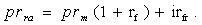 | (6) |
where, rf – the value of the nominal risk-free rate.If we decompose the real interest rate rr in expression (1) into the risk-free real rate and the (net of inflation) risk premium (prextrar)1 , the following transformation of the expression obtains: For the additive decomposition of the real rate (rr = rfr + prextrara):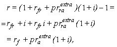 | (1a) |
For the multiplicative decomposition of the real rate 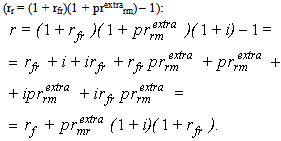 | (1b) |
The last components in expressions (1a) and (1b) are the observed (ex ante) risk-premia for the respective (i.e. additive or multiplicative) models. These expressions show that the inflation exerts immediate influence on the ex-ante risk premium. Moreover, Expression (1b) indicates that the ex-ante risk premium is also affected by the value of the implied real risk-free rate.
1.1. Interest Rate Algebra -1 (IRA-1)
Expressions (1a) and (1b) demonstrate that the detailed study of the subject of interest rates leads to realization that the number of structural representations for interest rates is not exhausted merely by the expressions (1)-(4). This is due to the following factors:• A risk-free rate can be represented either in nominal (rf) or real (rfr) terms;• A risk-free rate may either include some residual risk elements (rf and rfr), or be netted of any such elements (rnf and rnfr);• The risk premium can be represented differently for the additive (pra) or multiplicative (prm) interest rate models;• The risk premium can be represented in nominal (pr) or real (prr) terms;• The risk premium can be used in conjunction with “risk-free rates” which incorporate some residual risk elements - rf, rfr (in this case the risk premium shall be denoted with the “extra” superscript prextra), as well as in conjunction with absolute (“pure”) risk-free rates - rnf, rnfr (in this case, the notation for such risk premia does without the «extra» superscript - pr). Having regard to these circumstances, an attempt is made below to list all possible detailed specifications of the interest rate structure, which can be employed in the context of discounting for risky cash flows (in situations where the risk factor is incorporated in the discount rates, and not through adjusting the cash flows themselves, as the case may be): | (7) |
 | (8) |
 | (9) |
 | (10) |
 | (11) |
 | (12) |
 | (13) |
 | (14) |
 | (15) |
 | (16) |
 | (17) |
 | (18) |
 | (19) |
 | (20) |
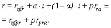
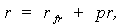
where:r – the nominal rate of interest/return that accounts for risks,rnfr - pure real risk-free rate (i.e. one net of all risks and inflation),rnf – pure nominal risk-free rate,i – the rate of inflation,rf – nominal risk-free rate, that includes some residual elements of risk in practical terms (residual risk elements),rfr – real risk-free rate with some residual risk elements,prrm – full risk premium in the multiplicative representation, net of inflation,prm – full risk premium in the multiplicative representation, incorporating inflation,prra – full risk premium in the additive representation, net of inflation,pra – full risk premium in the additive representation, incorporating inflation,prextram – partial risk premium over and above the residual risk elements in the risk-free rate rf , in the multiplicative representation (incorporating inflation),prextrarm – partial risk premium over and above the residual risk elements in the risk-free rate rf , in the multiplicative representation (net of inflation),prextraa - partial risk premium over and above the residual risk elements in the risk-free rate rf , in the additive representation (incorporating inflation),prextrara – partial risk premium over and above the residual risk elements in the risk-free rate rf , in the additive representation (net of inflation),rfpr – risk-free rate with partial account for inflation: rfpr = rfr + αi ,rnfpr – pure risk-free rate with partial account for inflation: rnfpr = rnfr + αi ,prextrapra – partial risk premium over and above the residual risk elements in the risk-free rate rfpr , in the additive representation (with partial account for inflation): prextrapra= prextrara + (1 - α)i, prpra – risk premium with a partial account for inflation applicable in the additive models and to be used in conjunction with the rnfpr risk-free rate partially accounting for inflation: prpra = prra + (1 - α)i ,α – a share (fraction) of inflation reflected (included) in the risk-free rate, 0 ≤ α ≤ 1,(1 – α) – the remaining share (fraction) of inflation reflected (included) in the risk premium.It can be ascertained that Models in (19) and (20) reflect valid options for inflation accounting -- both in relation to the risk-free rate and the risk premium.
1.2. Interest Rate Algebra -2 (IRA-2)
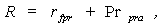
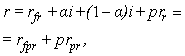
As the dealings in actual professional practice are for the most part limited to the observed “risk-free” rates which contain (or may contain) the admixtures of risk elements (in other words, we have no data on the values of pure risk-free market interest rates rnfr and rnf), practical value attaches only to those Expressions, out of the set of Expressions (6)-( 19), which do not contain pure risk-free rates (rnfr and rnf), i.e. to Expressions (9)-(11), (14)-(15), (17)-(18). Since all these Expressions carry the “extra” superscript in the notation for risk premia, it now makes sense to do away with using this superscript for sheer practicality. To avoid confusion in what follows, let us make use of a new notation, removing the “extra” superscript and replacing lower-case letters with the capital ones (it is possible, of course, to continue with using the lower-case letters -- bearing in mind that the applicable value of the risk premium is only partial, as some of its elements have actually been “woven” into the practically observed equivalent for the risk-free rate): | (21) |
 | (22) |
 | (23) |
 | (24) |
 | (25) |
 | (26) |
 | (27) |
where, R is an equivalent of r , Pr – of praextra , and Prpra – of prpraextra in terms of notation previously employed in the Expressions (7)-(20).As seen from the above expressions, IRA-2 assumes a complete absence of risk elements in the risk-free rate. This option algebra, as well as IRA-1, allows for the possibility of presentation of models for valuing the discount rate in multiplicative and additive forms.
1.3. Interest Rate Algebra -3 (IRA-3)
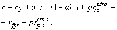
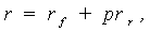
Having regard to the fact that appraisers and investment analysts for the most part limit themselves to the consideration of additive-type interest rate models, the immediately preceding algebra of interest rates (IRA-2) can be further simplified by excluding from it all the multiplicative-type models and leaving in only the additive models. Simultaneously, with the multiplicative models no longer featuring in the algebra, we shall exclude from the ensuing expressions all “a” subscripts denoting the membership in the additive-type model class. As a result, this new, simplest, algebra set features only additive models in the following representations: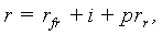 | (28) |
 | (29) |
 | (30) |
 | (31) |
where r is the equivalent of R, prr - of Prra, pr - of Prra, prpr - of Prpra in terms of notation previously used in the Expressions (21) – (23), (27), namely:r – is the nominal rate of interest applicable for discounting after-tax cash flows from a risky investment project (risky cash flows),rfr – real (i.e. net of inflation) risk-free interest rate (essentially reflecting the above mentioned “usurious” (i.e. “net-net-net”) interest), prr – real (net of inflation) risk premium,pr – nominal risk premium that includes the inflationary component,ά – a share (fraction) of inflation included (reflected) in the risk-free rate rfpr,(1 - ά) – the remaining share (fraction) of inflation included (reflected) in the risk premium prpr.As seen from the above expressions, in the General case, inflation can be taken into account as the risk-free rate and the risk premium. However, it is important to avoid double counting: in other words, inflation can only redistribute between the risk-free rate and a risk premium.
2. Accounting for Default and Insolvency Risks
Let us now take up the subject of the impact of risk on discount rates from a different standpoint. The lack-of-arbitrage-opportunities condition can be expressed as follows: | (32) |
where, pd – probability of insolvency/default (or, of a shortfall in payments, put simply), k – losses given default (as a fraction of the amount outstanding), rf – risk-free rate, r1 – expected return on investment into shares, at a favorable outcome. On the basis of Expression (32), it is possible to obtain an expression linking the above-mentioned expected return with the risk-free rate and the parameters of risk: | (33) |
Expression (33), in turn, is amenable for the quantification of the risk premium:-given the additive specification for the risk-free rate and the risk premium: | (34) |
- given the multiplicative specification for the risk-free rate and the risk premium: | (35) |
On the other hand, the relation between the risky rate and risk parameters can be obtained from a different consideration: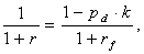 | (36) |
where, the numerator in the right-hand side of this equation reflects the adjustment to expected cash flows that transforms them into their certainty equivalents. Solving Equation (36) for r results in the following expression for the risky rate: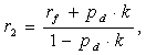 | (37) |
where r2 – is the estimate for risky rate obtained on the basis of Condition (36).Expression (37) also allows for deriving an expression for the risk premium:- for the additive relation between the risk-free rate and the risk premium: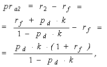 | (38) |
- for the multiplicative relation between the risk-free rate and the risk premium: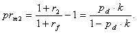 | (39) |
Despite their similarity, The Expressions (33) and (37) are not identical. The author of this Paper is hard put to give a conclusive explanation to the disparity between the formulas, however, it can be assumed that its nature is associated with the fact that in real life the number of possible event scenarios is significantly above the two outcomes implied in the initial lack-of-arbitrage hypothesis. In this regard, and as of the writing, there is a reason to repose greater trust in the Expression (37). Subsequent to deriving these formulas, the author of this Paper found in the literature[6]2 an expression similar (even to the point of notation) to one in (33), which, as suggested in the source, can be used for estimating returns on risky bonds. The respective passage from the work of W. Sharpe is reproduced below: “How high should a default risk premium be for a bond? According to one model [7], the answer depends both on the probability of default and on the possible financial losses of bondholders given the default. Consider a bond whose probability of default is constant every year (provided that the payments for previous years have been met). Let the probability of default during a given year be denoted as pd. Assume that, if the payments are remiss on the bond, the owner of each bond recovers a part, equal (1 - λ), of its market price in effect a year ago. According to this model, the bond shall be fairly priced, if its yield to maturity, “y”, equals to: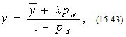 | (40) |
where, y denotes the expected yield to maturity of the bond. The difference, d, between the expected yield to maturity “y” and the expected [baseline] yield y has been previously alluded to as the default risk premium. Using the expression (15.4), we can see that this difference for fairly priced bonds should be equal to: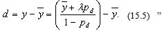 | (41) |
(end of the quote).In conclusion, it bears mentioning that cash flow discounting can be exercised in one of the two following ways:• Each period payment is discounted using a discount rate specific to that period;• A single discount rate is used for all periods - which corresponds to the “duration” of expected cash flows. The problem encountered with this approach is the difficulty of giving simultaneous/summary estimation to a set of rates in the form of an average expected interest rate (scoping over the investment horizon) – estimation which would not fail to reflect all the possible risks in the capital market.
3. Conclusions
On a final note, it is necessary to sum up the principal point covered in this paper.• First of all, the inflation exerts immediate influence on the ex-ante risk premium (see Expressions (1a), (1b));• Secondly, it should be noted that ex-ante risk premium is also affected by the value of the implied real risk-free rate (see Expression (1b));• Thirdly, the relationship between the discount rate and the risk has non-linear character (see Expressions (33), (37));• Finally, model estimates of the risk premium should correspond to the applied model of the calculation of the risk discount rate (see Expressions (34), (35), (38), (39)).Received in this article the results can hope to reach a more accurate calculations and the avoidance of errors in estimating discount rates.
Notes
1. To avoid double-counting in practical terms, only that part of the risk premium (prextrara) is to be accounted for in this exercise which is not already implicitly assumed in the risk-free rate, since risk-free rate metrics used in practice, arguably, admit of the presence of a small element of risk in them. 2. In W. Sharpe “Investments” (Russian edition, by Infra-M Publishers, Moscow, 2007). pp. 432-433, at the point where the work of Gordon Pye (Gordon Pye «Gauging the Default Premium», Financial Analysts Journal, 30, no.1 (January/February 1974), pp. 423-434) is being referenced.
References
| [1] | Irving Fisher, “The Theory of Interest”, New York: Macmillan, 1930. |
| [2] | William F. Sharpe “Capital Asset Prices: A Theory of Market Equilibrium Under Conditions of Risk”, Journal of Finance, 19, no.3 (September 1964), pp.425-442. |
| [3] | John Lintner, “The Valuation of Risk Assets and Selection of Risky Investments in Stock Portfolios and Capital Budgets”, Review of Economics and Statistics, 47, no.1 (February 1965), pp.13-37. |
| [4] | John Lintner, “Security Prices, Risk, and Maximal Gains from Deversification”, Journal of Finance, 20, no. 4 (December 1965), pp. 587-615. |
| [5] | Jan Mossin, “Equilibrium in a Capital Asset Market”, Econometrica, 34, no.4 (October 1966), pp.768-783. |
| [6] | William F. Sharpe, Gordon J.Alexander, Jeffery V. Bailey “Investments”, 5th ed., Prentice Hall International, Inc., USA, 1995 (Russian edition, by Infra-M Publishers, Moscow, 1997, pp. 432-433). |
| [7] | Gordon Pye, «Gauging the Default Premium», Financial Analysts Journal, 30, no.1 (January/February 1974), pp. 423-434. |
 Abstract
 Reference
 Full-Text PDF
 Full-text HTML