1. Introduction

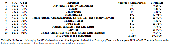
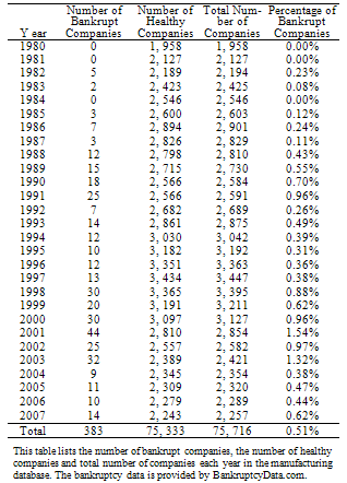
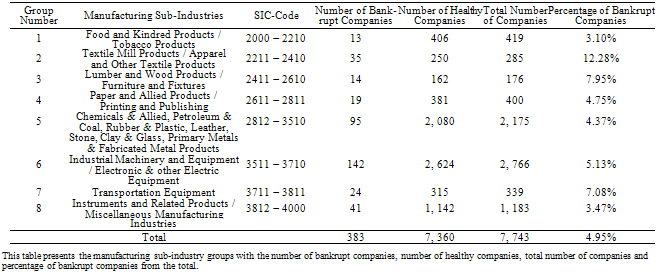
As the center of economic activity, the manufacturing industry is crucial to every economy as a source of productivity, higher standard of living, innovation, and the ability to compete on international ground. In addition, the manufacturing sector accounts for a major part of the GDP and employment in the United States. It is deeply interwoven with other industries that either depends on the products produced by the manufacturing industry, or with suppliers that provide the manufacturing industry with their products, raw materials, and services. The intense interaction with other industries and the major contribution to the U.S. GDP, output, and employment makes the manufacturing sector a substantially important industry for the U.S. economy. The vulnerability and the significance of the manufacturing industry to the U.S. make us aware of the importance of avoiding corporate bankruptcy and forecasting bankruptcy in the manufacturing sector, especially in the current economic situation.

US economy is experiencing the worst economic and financial crisis since the Great Depression of the 1930s. It is characterized by subprime housing crisis, increasing unemployment, low interest rates, and bankruptcies throughout all industries. Firms in every industry, but especially the manufacturing industry are struggling to survive decreasing demand, increasing unemployment and heavy debt burdens. Table 1 shows that the highest number of bankruptcies occur in the manufacturing industry. There are 802 bankruptcies in this sector, which represents 35% of all bankruptcy filings from 1978 to 2007. Throughout history we have seen the manufacturing industry suffering most under economic downturns. The bankruptcy data from BankruptcyData.com in Table 2 reports the highest number of bankruptcy filings between the years 2000 and 2003 as a result of the economic crisis in mid-2000. Unfortunately, the current recession that started in 2008 with the financial crisis hit the manufacturing industry again. Many manufacturing firms have filed for bankruptcy since the beginning of the crisis. BankruptcyData.com reports among other manufacturing companies the giant manufacturer of chemicals Lyondell Chemical Company (with an asset value of $ 27,392 million and over 16,000 employees worldwide) which filed for Chapter 11 bankruptcy in January 2009. Another major company that filed for Chapter 11 bankruptcy in April 2009 is the producer of newsprint Abitibi Bowater Inc with an asset value of $ 10,319 million. However, the most affected industry is the automobile industry that according to the Bureau of Labor Statistics employs more than 7 Million employees. Automobile companies like General Motors and Chrysler have been struggling with declining demand and debt burdens since the beginning of the economic crisis. Despite huge bailouts, one of the giant automobile producers, Chrysler was finally forced to file for Chapter 11 bankruptcy protection at the end of April 2009.

Forecasting bankruptcy is important for many different interest groups like private investors, the financial sector, corporations, employees, and the government. Each group represents different interests and stakes. Private investors, shareholders and banks try to reduce the risk of losing their investments in case of default. On the other hand, there are firm insiders and stakeholders like managers who try to maximize shareholder and stakeholder value, as well as their own income. Other important interest groups are the government and employees that are particularly interested in tools that enable bankruptcy prediction in order to avoid unemployment, economic distress, inflation and a declining Gross Domestic Product (GDP). In addition, there is a huge interest in finding an applicable bankruptcy prediction model from an academic point of view. Authors who analyzed bankruptcy have used accounting driven or market driven variables with static or hazard models in order to predict bankruptcy. Since the mid-1960s many authors have approached the question of forecasting bankruptcy through firm specific accounting variables. Ratios that reflect Solvency, Liquidity and Leverage are the most analyzed variables. Beaver[3], Altman[4], Ohlson[5], and Zmijewski[6] were some of the first authors who tried to forecast bankruptcy through financial statement ratios. More recent authors like Core and Schrand[7], Duffie and Lando[8], and Shumway[9] argue that accounting variables are not sufficient for analyzing bankruptcy and suggest that market driven variables or a mix of financial statement ratios and market driven variables are better bankruptcy forecasters. Shumway[9] shows in his hazard analysis that market driven variables are better bankruptcy predictors and that half of the financial ratios used by previous authors are not significant in predicting bankruptcy. This result is supported by other authors like Chava & Jarrow[10] and Hillegeist et al.[11].

This paper will contribute to the existing bankruptcy literature by analyzing the manufacturing industry and by adding the macroeconomic variable GDP to the bankruptcy prediction model. As shortly explained in section 1.1, the manufacturing sector is a significant industry in the U.S., it does not only contribute substantially to the U.S. GDP but it also depends on a stable GDP and a sound economy. In the past we have seen the manufacturing sector suffering from economic downturns and decreasing GDP, therefore we expect a correlation between the GDP rate and bankruptcy filings in the manufacturing industry.[1]

In fact, the results in this paper show that GDP is a significant bankruptcy predictor in the manufacturing industry. In addition, the results support the superiority of market variables over accounting variables for predicting bankruptcy. The only significant variable among the accounting variables is the liquidity ratio current assets to current liability. After applying a model that combines accounting, market, and macroeconomic variables to the whole manufacturing sector and to the sub-industries of the manufacturing sector we find the following results: All four variables (CACL, EXRET, SIGMA and changeGDP) are significant in predicting bankruptcy in the whole manufacturing industry. In the analysis of the manufacturing sub-industries the excess return of companies over the S&P500 return is a significant bankruptcy predictor in 7 of the 8 manufacturing sub-industries. GDP is significant in the industrial machinery industry and liquidity is significant in the textile and chemicals industry.

This paper consists of five parts. After the introduction, the second part reviews the contribution of previous authors to the bankruptcy forecasting literature. The third part describes the data and sources used for this paper. The fourth part will explain the methodology and the bankruptcy predicting variables. Part five will discuss the results of the bankruptcy prediction and the final part will summarize the results.

1.1. The Importance of the Manufacturing Industry for the U.S. Economy

In 2007, the U.S. manufacturing sector accounted for 11.5% of the GDP, 20% of the gross output and almost 10% of US employment (mainly to blue-collar workers but also to white-collar employees). However, the manufacturing sector is not only an important provider of employment and producer of innovative end-products benefiting the consumer; it is also in the center of the productivity chain. It is a major producer of intermediate goods and a major demander of raw materials, goods, and services from many industries. The manufacturing sector accounts for 28% (a total value of 3,417.1 Billion US-Dollar) of intermediate inputs produced in the U.S. in 2008, which is the highest percentage compared to other industries intermediate input. The U.S. manufacturing industry belongs to the world’s leading producer of manufacturing products with increasing productivity. According to an economic release of the Bureau of Labor Statistics in March 2009, the U.S. labor productivity in manufacturing increased 4.7% over the period of 2006 to 2007 representing the fourth largest productivity growth of 14 economies. Over the same period, labor costs have been declining in the U.S. by 1.1 %.

The current economy will depend increasingly on the success of the manufacturing industry due to the declining finance, insurance and real estate industries. Long term economic stability, international competitiveness, innovation and increasing standards of living depend on a growing manufacturing sector. The challenges of international competitiveness are increasing with improved technology, reduction of barriers to trade such as tariffs and quotas in the last few decades, and the rising of new competitors such as China, Taiwan, and Korea. The key to stable and competitive manufacturing is innovation, which is the driving factor for increasing productivity. An increasing productivity improves the standard of living through increasing wages and lower prices for better quality. Because of the major impact of the manufacturing sector on a stable U.S. economy and the overall standards of living it is especially more important to avoid bankruptcy within this sector.

2. Literature Review

The first authors who analyzed bankruptcy prediction focused on finding the optimal accounting variables to predict bankruptcy. Authors like Beaver[3], Altman[4], Ohlson[5], and Zmijewski[6] used a static model to predict bankruptcy through accounting variables. More recent authors like Shumway[9], Campbell et al.[13], and Chava and Jarrow[10] used a logit model to predict bankruptcy. Shumway[9] proposed the hazard model and illustrates in his work the drawbacks of the static models used by the previous authors. He argues that the static model introduces a bias and causes an overestimation of the bankruptcy determinants. These recent authors who discovered stock market information as important predictors discussed the superiority of the two different types of bankruptcy prediction sources. Some authors argue that accounting information is not significant or incremental in supporting market driven variables, other authors suggest that accounting variables are incremental in forecasting bankruptcy.

Altman[4] analyzed the significance of five financial ratios (Working Capital /Total Assets (WC/TA), Retained Earnings/Total Assets (RE/TA), Earnings Before Interest and Tax/Total Assets (EBIT/TA), Market Value of Equity/Total Liabilities (ME/TL), and Sales/Total Assets(S/TA)) in forecasting bankruptcy with a rather small sample of 66 manufacturing firms. He applied his famous Z-Score which is still used to predict bankruptcy in the short run (one to two years) by many market professionals. He found that all ratios deteriorated as the sample companies came closer to the bankruptcy year. As the Z-Score decreases to 1.8 or less, the probability of bankruptcy is very high, while a Z-Score of 3.0 or higher predicts a lower risk for bankruptcy. His Multiple Discriminant Model was accurate in forecasting bankruptcy up to two years before bankruptcy.

Beaver[3] approached bankruptcy prediction by pairing each bankrupt firm with a non-bankrupt firm in the same industry and with the same asset size in order to account for industry and size effects. His non-random sample contained 79 sample pairs from 38 different industries. Beaver[3] analyzed the predictability of bankruptcy through the following six financial ratios: Cash Flow/Total Debt(CF/TA), Net Income/Total Assets(NI/TA), Total Debt/Total Assets(TD/TA), Working Capital/Total Assets(WC/TA), CR and No-credit interval. From the six ratios he analyzed, the Cash Flow to Total Debt ratio turned out to be the strongest bankruptcy predictor.

Ohlson[5] developed a model with nine variables: Size, Total Liabilities/Total Assets (TL/TA), Working Capital/Total Assets (WC/TA), Current Liabilities/Current Assets (CL/CA), OENEG, Net Income/Total Assets (NI/TA), FU/TL, INTWO, and CHIN. His sample contained 2,058 non- bankrupt firms and 105 bankrupt firms. He found that four of his nine variables were significant in forecasting bankruptcy; Size, Total Liabilities/Total Assets (TL/TA), Net Income/Total Assets(NI/TA), and Working Capital/Total Assets(WC/TA).

In 1984, Zmijewski[6] argued in his analysis of bankruptcy prediction, that non- random samples would increase the bias in parameter and probability. He analyzed the following three accounting variables; return on assets which is the ratio of Net Income to Total Assets (NI/TA), the current ratio Current Assets to Current Liability (CA/CL) and Total Liability to Total Assets (TL/TA).

Shumway[9] criticizes the static models used by previous authors as biased models and suggests an unbiased and consistent hazard model based on authors like Theodossiou[12] who proposes a dynamic model of bankruptcy prediction. The hazard model accounts for many factors for which static models were not able to account for. Shumway[9] argues that hazard models account for endangered periods before filing for bankruptcy, time-series fluctuation in the data and better performance in out-of-sample prediction due to independent observations. Shumway[9] adds the variable firm size as the market capitalization of each firm relative to the NYSE/AMEX market size, past excess stock returns as the difference between each company’s return and the NYSE/ AMEX index return and the idiosyncratic standard deviation of stock returns as market driven variables to the traditional financial statement ratios used in the analysis of Altman[4] and Zmijewski[6]. By applying his hazard model (with a sample extending from 1962 to 1992, 39,745 firm-years and 300 bankruptcies) he finds that from the five Altman[4] accounting variables only EBIT/TA and ME/TL are significant in forecasting bankruptcy and only one independent variable (NI/TA) from the original three Zmijewski[6] variables are significant in forecasting bankruptcy. His market driven variables model and the mixed model of market driven and accounting variables perform best in predicting failure. His mixed hazard model turns out to be a better out-of-sample test than the concentration on accounting variables or market variables only.

Shumway[9] s results are supported by Hillegeist et al.[11] who challenge Altman[4] s Z-Score and Ohlson[5] s O-Score with a large sample of 65,960 firm year observations containing 516 bankruptcies for the years 1979 to 1997. These authors combine Altman[4]s Z-Score and Ohlson[5]s O-Score with option-pricing theories suggested by Black and Scholes and Merton which argue that accounting variables do not contribute significantly in predicting bankruptcy and that stock market variables are better bankruptcy predictors. The conclusion of Hillegeist et al.[11] s analysis is that relying only on accounting variables for bankruptcy prediction such as the Z- Score and O-Score is not adequate. However, these scores add significant information to the prediction with market variables.

Other authors analyzing a mix of stock market and accounting variables are Campbell et al.[13]. These authors consider in their study not only firms that actually filed for Chapter 7 or Chapter 11 bankruptcy but also firms which are delisted by credit rating agencies. Campbell et al.[13] follow bankruptcy analysis models of previous authors like Shumway[9] and Chava and Jarrow[10] with the use of a dynamic logit model and monthly bankruptcy indicators (for 1.7 million firm months) from January 1963 to December 1998 for firms which filed for Chapter 7 or Chapter 11 bankruptcy. The second set of data contains not only Chapter 7 and Chapter 11 filings but delisting or D ratings spanning from January 1996 to December 2003. Campbell et al.[13] analyze some of the variables previously used by authors like Shumway[9] like NI/TA and TL/TA; however, the authors use the market value of Total Assets instead of the book value and add some additional market variables like EXRET, SIGMA, RSIZE, and PRIZE to the variables used by previous authors which add up to a total of ten variables with NIMTA, TLMTA, CASHMTA and MB.

Chava and Jarrow[10] support Shumway[9] s model and add industry effects to their bankruptcy analysis with a data set that expands from 1962 to 1999. These authors not only add the industrial effect to the work of previous authors, but also expand the bankruptcy literature with data on financial institutions. First Chava & Jarrow[10] re-estimate the work of Altman[4], Zmijewski[6] and Shumway[9] and confirm the outperforming power of Shumway[9] s hazard model (74.4% of bankruptcies correctly identified) compared to the static model with accounting variables only which were used by Altman[4] (63.2%) and Zmijewski[6] (43.2%). Second, the authors prove the importance of industry effect on in-sample accuracy in bankruptcy prediction. Next, the previous literature is expanded by data on the financial industry and the authors show that prediction power improves using monthly data versus yearly data used by most of the previous authors. In the last part of the analysis, Chava & Jarrow[10] show that accounting variables contribute to forecasting power when market variables are already accounted for.

3. Data

There are two major bankruptcy codes in the United States; Chapter 7 and Chapter 11 bankruptcy. Companies that cannot pay their debts when they become due can first try to settle an informal agreement with their debt holders. However, for large companies with complex capital structure an informal agreement is difficult to settle; therefore, large firms end up filing for either Chapter 7 or Chapter 11 bankruptcy. The keyword for Chapter 7 bankruptcy is liquidation. In this case the assets of the company filing for Chapter 7 bankruptcy are liquidated by a trustee in order to distribute the proceeds to the creditors. The proceeds are used in a certain order to pay off debt[1,2].

The bankruptcy code Chapter 11 is a reorganization of the company and its capital structure rather than an immediate liquidation. The company’s management is expected to provide a plan of reorganization within 120 days after bankruptcy filing so that the company can continue to operate and perhaps survive the bankruptcy. The advantage of filing for Chapter 11 rather than Chapter 7 bankruptcy for the management is that it does not have to give up the control of the company to a trustee. Chapter 11 is not only advantageous for the management but also for the government, employees and shareholders. If the company survives, unemployment is avoided which is positive for the government and employees and shareholders of the company do not lose their investment.

For this paper, a company is defined as bankrupt if it filed either for Chapter 7 or Chapter 11 bankruptcy. Because of financial and liquidation uncertainties which lead to a Chapter 11 bankruptcy, these filings will be included in the bankruptcy definition, although Chapter 11 bankruptcy does not necessarily lead to a liquidation of the company through a Chapter 7 filing.

The bankruptcy information is obtained from BankruptcyData.com, containing a total of 2,286 bankruptcies in all industries from 1978 to 2007. Table 1 shows that the highest number of bankruptcies occur in the manufacturing industry. There are 802 bankruptcies in this sector, which represent 35% of all bankruptcy filings. Table 2 shows the per year number of bankrupt and healthy companies for our database on the manufacturing industry from 1980 to 2000. The highest number and percentage of bankruptcy filings occur in the years of 2000 to 2003 as a result of the economic recession in mid-2000.

For the bankruptcy forecasting model balance sheet and income statement values are obtained from the COMPUSTAT database and market values are obtained from the CRSP database. CRSP and COMPUSTAT include public companies traded on the NYSE and AMEX from 1980 to 2007. These databases are reduced to manufacturing companies with SIC-Codes 2000 and 4000. As the macroeconomic indicator quarterly real percentage changes in GDP from 1980 to 2007 are obtained from the Bureau of Economic Analysis.

Table 1. Bankruptcy by Industry

After merging quarterly COMPUSTAT observations with monthly CRSP observations and the bankruptcy filings our complete dataset contains 845,587 firm month observations, 7,743 firms and 383 bankruptcies (5%). All the companies in our analysis are publicly traded companies. Since we do not have proper financial statement information for private companies they are not included in our study. Missing observations in the database are replaced by previous period observations.

Table 2. Bankruptcy the Manufacturing Industry by Year

The bankruptcy indicator in this paper equals 1 if the company filed for bankruptcy and 0 for companies which have not filed for bankruptcy or have disappeared from the database due to merger and acquisition. Companies which have been delisted up to five years before filing for bankruptcy are considered as bankrupt as well. For all companies that filed for bankruptcy, all observations after the bankruptcy filing date are deleted from the database.

4. Variables and Methodology

4.1. Dependent Variable

The dependent variable bankrupt is a binary variable. It equals 1 if the company filed for bankruptcy in a particular month and 0 if not. For companies which have been overtaken by another company or have merged, the dependent variable is equal to zero as well.

4.2. Independent Variables

The following five accounting variables for this paper are chosen from Altman[4]. The first determinant is the liquidity ratio Working Capital to Total Assets (WCTA); it compares the liquid assets of a firm to its total assets. An increase in WCTA translates to a higher or improving liquidity of the firm. On the other hand, a failing company is more likely to experience a decrease in current assets through loses, causing a decreasing WCTA. Retained Earnings to Total Assets (RETA) will enter the analysis as a profitability ratio which shows how much a company is able to retain from its earnings through the use of the assets. The third variable is Earnings Before Interest and Tax to Total Assets (EBITTA), also known as Return on Assets. An increasing EBITTA shows that the company is able to generate more income with its assets. Although early authors like Altman[4] concentrated more on accounting variables rather than market variables, Market Equity to Total Liability (METL) implied a market dimension to his analysis. Market equity is equal to the price per share times the number of shares outstanding. METL relates the market value of the company to its total liabilities. For a sound company we expect a high or increasing METL, while a failing company is more likely to have a decreasing METL. The last bankruptcy determinant is the asset turnover ratio Sales to Total Assets (STA). Since sales were not available in the COMPUSTAT database, the Sales to Total Assets ratio is replaced by the Revenue to Total Assets (RTA) ratio in this paper. This measure shows how much revenue each dollar of a firms assets can produce. A decreasing RTA indicates a slowdown of production, while a high or increasing RTA compared to the industry average indicates increasing production or production close to capacity [14,15].

The following three accounting variables analyzed in this paper come from Zmijewski[6] s model: Net Income to Total Assets (NITA), Total Liability to Total Assets (TLTA) and Current assets to Current Liabilities (CACL).

NITA, a profitability ratio, shows how efficient total assets are used to generate earnings. The leverage ratio Total Liabilities to Total Assets measures how many percent of the company’s assets are financed through liabilities. Since high level of liabilities are associated with higher risk, we expect the debt ratio to be high or increasing for failing companies and low or decreasing levels of TLTA for stable companies. The third Zmijewski[6] variable is Current Assets to Current Liability; another liquidity ratio showing how much assets are available for each dollar in Current Liabilities.

The market variables analyzed in this paper are relative size of the firm (RSIZE), excess return (EXRET), and the standard deviation of each firms return (SIGMA). RSIZE is calculated as the ratio of market capitalization of the firm to the total market size of the manufacturing market. EXRET is computed as the difference between the firms return and the value weighted S&P 500 return from the CRSP dataset. The third market variable SIGMA is the standard deviation of the returns, indicating the volatility in returns. These determinants were first introduced by Shumway[9] and later reanalyzed by Chava and Jarrow[10] and Campbell et al.[13]. Shumway[9] argues and finds that Firm Size (RSIZE), Excess Returns (EXRET) and SIGMA are important for bankruptcy analysis.

The new variable introduced in this paper is the percentage change in real GDP (changeGDP) compared to the previous quarter. This variable enters the model as a macroeconomic indicator for bankruptcy. We expect decreasing bankruptcy filings for an increase in the change of GDP.

An overview of the ratios used for the models in this paper is available in the appendix.

5. Methodology

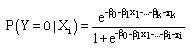
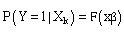
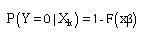
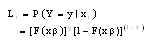
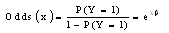
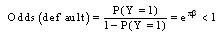
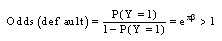
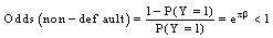
Multi-period logistic regression or hazard models enable the prediction of the outcome of a certain event for a given set of independent variables. The advantages of the hazard rate model will be used in this paper in order to predict if a company will survive or fail given monthly firm observations. The advantage of the hazard model is that it explicitly accounts for time and it incorporates time-varying covariates. In a hazard model, a firm’s risk of bankruptcy changes through time based on its latest financial data.

The dependent variable Y in this study is a binary variable. For this purpose, we created the variable bankrupt which can take only two values for each firm-month i at the time t = 1, , n. The dependent variable y_i is equal to 1 if a company files for bankruptcy in month t and 0 otherwise. However, y_i = 0 can occur either for the case healthy company or company leaves the sample for other reasons like merger or acquisition. Each company’s observation months are assumed to be independent. Therefore the age of the company cannot be an indicator for risk.[16]

The logistic distribution is given as follows:

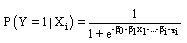(1)

(2)

(3)

where xi s are the explanatory variables and βi s are the unknown parameters to be estimated. The regression function β0 + β1x1 + ... + βi xi will be written as xβ.

The coefficients of the logistic regression are estimated using the maximum likelihood function.

(4)

(5)

(6)

The estimated coefficients in this paper will be interpreted in the form of odds ratios. The odds of failure is the probability that a company goes bankrupt divided by the probability that the company does not go bankrupt:

(7)

(8)

The logistic regression presents the odds ratio of bankruptcy. The interpretation of odds ratios for bankruptcy prediction is as follows:

(9)

Odds ratios smaller than 1 decrease the odds of default.

(10)

Odds ratios larger than 1 increase the odds of default. The odds of non-default is defined as follows:

(11)

Odds ratios smaller than 1 decrease the odds of non-default.

(12)

Odds ratios larger than 1 increase the odds of non-default.

Table 3. Manufacturing Sub-Industries

Table 4. Odds Ratio of Non-Default to Default for Default Models

The results of the multi-period logistic model on the bankruptcy predictors will be reported in odds of non-default in Tables 4 and 5.

6. Results

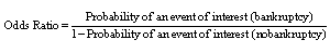
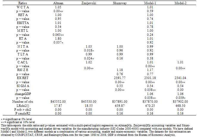
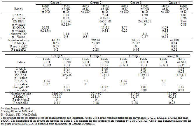
This section analyzes the odds ratio and p-value estimates for various models (under the ceteris paribus assumption). First, the validity of previous authors forecasting models is tested with the database of the manufacturing sector. For this purpose, Altman[4] s and Zmijewski[6] s accounting variables and Shumway[9] s market variables are used to estimate odds ratios and p-values for the manufacturing database for the years 1980 to 2007. In addition, these models are re-estimated by adding the macroeconomic variable GDP to each model. Next, the variables which performed best throughout all models are combined to a new model. Finally, we estimate odds ratios and p-values for the sub-industries (listed in Table 3) of the manufacturing industry with the new model that combines accounting and market-driven variables and the macroeconomic variable, change in GDP in order to detect any differences within the sub-industries. For all models, the Table 4 will present the odds of non-default to default.

Model with Altman[4] s Accounting Variables

The first column in Table 4 replicate Altman[4] s model (WCTA, RETA, EBITTA, METL and RTA) with the data on the manufacturing industry with SIC-Codes 2000 to 4000 for the years 1980 to 2007. The WCTA is significant at any significance level and the odds of non-default increases by 5% for a one unit increase of WCTA. A one unit increase in METL increases the odds of non-default by .04%. Finally, the odds of non-default increases by 80% for a one unit increase in RTA. This ratio is significant at the 5% significance level. The ratios RETA and EBITTA are not significant in forecasting bankruptcy.

The odds ratios reported show that a higher liquidity (WCTA) and higher asset turnover ratios (RTA) increase the odds of non-default which translates into decreasing chance of bankruptcy. The odds of non-default increases also for companies with high market capitalization and low total liabilities.

Model with Zmijewski[6] s Accounting Variables

Zmijewski[6] s model is replicated in the second columns of Table 4. The odds of non-default increases by almost 3% for a 1 unit increase of NITA. This ratio is significant at the 5% level. A one unit increase in TLTA increases the odds of default by 0.8% and is also significant at the 5% level. The last ratio of Zmijewski[6] s model is the liquidity ratio CACL. For a one unit increase in CACL, the odds of non-default increases by 1.5%. This ratio is significant at any significance level.

Zmijewski[6] s variables are all significant in forecasting bankruptcy. Higher re- turn on assets (NITA) and higher liquidity (CACL) decrease the risk of bankruptcy, while higher leverage (TLTA) increases the chance of bankruptcy.

Model with Shumway[9] s Market-Driven Variables

The third column of Table 4 presents the market-driven variables RSIZE, EXRET, and SIGMA and the accounting variables NITA and TLTA for the manufacturing industry from 1980 to 2007. The market variable EXRET is statistically significant at any significance level, the odds of default to non-default is almost zero for a one unit increase in EXRET. SIGMA, the volatility indicator increases the odds of default by 87% for a one unit increase in the standard deviation of the returns. RSIZE turns out to be insignificant for predicting bankruptcy.

Two of the three market variables turn out to be statistically significant in forecasting bankruptcy. While higher volatility increases the probability of bankruptcy, the risk of bankruptcy is lower for companies with returns that are higher than the S&P 500 return.

The combination of accounting variables with market variables results in the insignificance of NITA and TLTA which were significant in the previous models. Accounting variables lose predicting power when market-driven variables are added to the regression.

Model 1 - Model with all accounting and market-driven variables and GDP

All accounting variables (WCTA, RETA, EBITTA, METL, RTA, NITA, TLTA, and CACL) and market-driven variables (RSIZE, EXRET, and SIGMA) from the previous models and the change in GDP are combined in the model presented in Table 4 (called Model 1). This combined model performs well with a Pseudo R- square of 0.1590. However, Table 4 shows that all accounting variables, except of CACL loose significance when combined with market and macroeconomic variables. The liquidity ratio CACL is significant at any significance level and increases the odds of non-default by 1.4% for a one unit increase in the CACL ratio. The market variable RSIZE is insignificant in forecasting bankruptcy like in all previous models. EXRET turns out to be significant again in this model. The odds of default to non-default is almost zero for a one unit increase in EXRET. The last two variables SIGMA and GDP are both significant at the 5% level. A one unit increase in SIGMA increases the odds of default by 86%. The macroeconomic variable changeGDP performs also very well in forecasting bankruptcy in this model. A 1% increase in GDP increases the odds of non-default by 6%.

In this combined model, higher liquidity, higher returns, and increasing GDP decrease the chance of bankruptcy, while higher volatilities in returns increase the chance of default.

Model 2 - Model with CACL, EXRET, SIGMA and GDP

The last model in Table 4 (called Model 2) combines those variables which performed best throughout all previous models to a new model containing CACL, EXRET, SIGMA and changeGDP. The Pseudo R-square is equal to 0.1584, which is very close to the Pseudo R-square of Model 1 that combined all accounting, market and macroeconomic variables. The p-values in Table 4 show that all variables enter the model as significant bankruptcy predictors. The liquidity ratio CACL increases the odds of non-default by 1.4% for a one unit increase in CACL. The odds of default to non-default for EXRET is almost zero for a one unit increase in EXRET. The third variable SIGMA increases the odds of default by 86% for a one unit increase in the standard deviation of the returns. The change in GDP increases the odds of non-default by 6 % for a 1% increase in GDP.

Higher liquidity, higher excess returns and increasing GDP decrease also in this model the chance of default. In contrast, increasing standard deviations of returns increase the default probability. The Pseudo R-square of Model 2 is 0.1584, which is very close to the Pseudo R-square of Model 1 (0.1590) with all accounting, market-driven and macroeconomic variables although it includes only one accounting variable (CACL). Since Model 2 is almost as powerful as Model 1 with almost equal Pseudo R-squares, we will use this model to analyze the sub-industries in the manufacturing industry.

Model with Accounting and Market variables and GDP for Manufacturing Sub- Industries

The manufacturing sub-industries are divided into eight groups presented in Table 3. Because of the significance throughout all estimated models CACL, EXRET, SIGMA and changeGDP are used to analyze the manufacturing sub-industries. Table 5 presents the results for the sub-industries. These results show in some cases major differences to the estimation on the whole manufacturing industry in Table 4 where all variables turned out to be significant.

Group #1: Food and Kindred Products / Tobacco Products

The first two columns of the first part of Table 5 present the results for group 1. The market driven variable EXRET performs well in the sub-industry 1 as well as in the regression on the whole manufacturing industry. It is significant on the 5% level and the odd of default to non-default is almost zero for a one unit increase in EXRET. The second market variable SIGMA is significant at the 10% significance level and the odds of default is 30.8 times higher than the odds of non-default for a one unit increase in SIGMA. The macroeconomic variable changeGDP and CACL do not perform very well in the food and tobacco industry and are statistically insignificant in predicting bankruptcy.

Group # 2: Textile Mill Products / Apparel and other Textile products

The liquidity indicator CACL turns out to be a good predictor of bankruptcy in this sub-industry. This variable is significant at the 5% level and the odds of non-default is 2.2 times higher than the odds of default. EXRET turns out to be also a good failure predictor for the sub-industry 2. This indicator is significant at any significance level and the odds of default to non-default is almost zero for a one unit increase in EXRET. In contrast to sub-industry 1, SIGMA is insignificant and does not perform well in bankruptcy prediction. The change in GDP turns out to be insignificant for this group as well.

Group # 3: Lumber and Wood Products / Furniture and Fixtures

EXRET continuous to perform as a good forecasting indicator in group 3, it is significant at any level and the odds of default to non-default is close to zero for a one unit increase of EXRET. The variables SIGMA, CACL, and changeGDP are statistically insignificant in forecasting bankruptcy for group 3.

Group # 4: Paper and Allied Products / Printing and Publishing

The model does not perform very well in predicting bankruptcy for group 4. All four variables are insignificant in predicting failure probability.

Group # 5: Chemicals and Allied Products - Fabricated Metal Products

The second part of Table 5 shows that two of the four bankruptcy indicators turn out to be significant in predicting bankruptcy for sub-industry 5. A one unit increase in liquidity increases the odds of non-default by 1.3%. Excess returns turn out to be a significant predictor as well. The odds default to non-default for this variable is close to zero for a one unit increase in EXRET. The last two variables SIGMA and change in GDP are statistically not significant in predicting bankruptcy for this sub group of the manufacturing industry.

Group # 6: Industrial Machinery and Equipment / Electronic & other Electric Equipment

The bankruptcy prediction model performs best in forecasting failure in sub- industry 6. EXRET performs here as well as in the previous sub-industries. SIGMA, the volatility indicator is significant and the odds of default is 3.1 times higher than the odds of non-default for a one unit increase in SIGMA. The macroeconomic variable turns out to be a good forecasting indicator for sub-industry 6. A 1% increase in the change of GDP increases the odds of non-default by 12%. The only variable which is not significant is the liquidity indicator CACL. The significance of GDP in forecasting bankruptcy in the industrial machinery and equipment sub-industry is due to the fact that the demand for new machinery and equipment decreases in times of economic distress and decreasing GDP. Companies tend to reduce investments in new machinery and equipment during times of recession or negative future prospects. The reduced demand for industrial machinery might cause increasing bankruptcies in this sub-industry. However, not only companies cut back during times of distress, households reduce their demand as well. The tendency of households to reduce purchases of electronic devises and equipment during economic downturns might causes failure in the electronic and electronic equipment industry.

Table 5. Model-2 on Sub-Industries of the Manufacturing Industry

Group # 7: Transportation Equipment

In the transportation industry only EXRET turns out to be a good failure predictor. For a one unit increase in EXRET the odds of failure to non-failure is close to zero. CACL, SIGMA and changeGDP are insignificant in predicting bankruptcy.

Group # 8: Instruments and Related Products / Miscellaneous Manufacturing Industries

The results of the last sub-group in Table 5 are similar to the result of the transportation industry. Only EXRET is a good predictor for failure. It decreases the bankruptcy probability with increasing returns.

7. Conclusions

The results in this paper show that the accounting variables developed by authors like Altman[4] and Zmijewski[6] loose significance when they are combined with market-driven variables and macroeconomic variables. The only accounting variable that turns out to be significant throughout all models and combinations in Table 4 is the liquidity ratio current assets to current liability. Two of the three market driven variables (EXRET and SIGMA) perform also very well in predicting bankruptcy throughout all models in Tables 4. The macroeconomic factor GDP which is introduced in this paper as a new forecasting variable turns out to be a significant indicator for bankruptcy prediction. The results show that increasing GDP reduces the risk of bankruptcy.

The results of the manufacturing sub-industries are different for each sub-industry. The combination of one accounting factor (CACL), two market factors (EXRET and SIGMA), and one macroeconomic factor (changeGDP) performs well in some sub- industries and poor in other sub-industries. EXRET performs well in almost all sub-industries. It is a significant bankruptcy forecaster and decreases the odds of bankruptcy with increasing returns. Although the variable GDP is significant in only one of the sub-industries, it is a significant bankruptcy predictor in the whole manufacturing industry and helps in the prediction of bankruptcy.