1. Introduction

Neural networks are a class of generalized nonlinear models inspired by studies of the human brain. Their main advantage is that they can approximate any nonlinear function to an arbitrary degree of accuracy with a suitable number of hidden units. Neural networks get their intelligence from learning process, and then this intelligence makes them have the capability of auto-adaptability, association and memory to perform certain tasks.

The task of knowledge extraction from data is to select mathematical description from data. But the required knowledge for designing of mathematical models or architecture of neural networks is not at the command of the users In mathematical statistics it is need to have a priori information about the structure of the mathematical model. In neural networks the user estimates this structure by choosing the number of layers, and the number and transfer functions of nodes of a neural network. This requires not only knowledge about the theory of neural networks, but also knowledge of the object's nature and time. Besides this the knowledge from systems theory about the systems modelled is not applicable without transformation into an object in the neural network world. But the rules of translation are usually unknown[4].

GMDH type neural networks can overcome these problems. It can pick out knowledge about object directly from data sampling. The GMDH is the inductive sorting-out method, which has advantages in the cases of rather complex objects, having no definite theory, particularly for the objects with fuzzy characteristics. GMDH algorithms found the only optimal model using full sorting-out of model-candidates and operation of evaluation of them, by external criteria of accuracy or difference types[1,2].

In this paper, a method of non-parametric approach to predict the gold price over time in different condition of market is used. MLFF neural network with back-propagation algorithm and GMDH neural network with genetic algorithms are briefly discussed, and they are used to make appropriate model for predicting the gas price of Henry Hub Gulf Coast Natural gas spot price. As input variables to the neural networks, we use price time series separately with 2 lags of the 5, 10, 15, 30, 35, 50 and 55-day moving average crossover. These two models are coded and implemented in Matlab software package.

The prime aim here is to find out dependence in gas price and also which neural network model does best in forecasting when the input parameters are little or great. The remainder of the paper is organized as follows. Section 2 describes the non-parametric modeling approach adopted here as per MLFF neural network with back-propagation algorithm and GMDH neural network with genetic algorithms which are briefly discussed. Section 3 discusses relevant concepts of the technical indicators used for the study. Empirical results are presented in Section 4 and concluding remarks in Section 5.

2. Modeling Using Neural Network

Artificial Neural Networks (ANN) is biologically inspired network based on the organization of neurons and decision making process in the human brain[1]. In other words, it is the mathematical analogue of the human nervous system. This can be used for prediction, pattern recognition and pattern classification purposes. It has been proved by several authors that ANN can be of great used when the associated system is so complex that the underline processes or relationship are not completely understandable or display chaotic properties[13]. Development of ANN model for any system involves three important issues: (i) topology of the network, (ii) a proper training algorithm and (iii) transfer function. Basically an ANN involves an input layer and an output layer connected through one or more hidden layers. The network learns by adjusting the inter connections between the layers. When the learning or training procedure is completed, a suitable output is produced at the output layer. The learning procedure may be supervised or unsupervised. In prediction problem supervised learning is adopted where a desired output is assigned to network before hand[14].

2.1. MLFF Neural Network

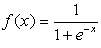
MLFF neural network is one the famous and it is used at more than 50 percent of researches that are doing in economy field recently[23]. This class of networks consists of multiple layers of computational units, usually interconnected in a feed-forward way. Each neuron in one layer has directed connections to the neurons of the subsequent layer. In many applications the units of these networks apply a sigmoid function as a transfer function (). It has a continuous derivative, which allows it to be used in back- propagation. This function is also preferred because its derivative is easily calculated:

Multi-layer networks use a variety of learning techniques; the most popular is back-propagation algorithm (BPA). The BPA is a supervised learning algorithm that aims at reducing overall system error to a minimum[1,9]. This algorithm has made multilayer neural networks suitable for various prediction problems. In this learning procedure, an initial weight vectors is updated according to[10]:

(1)

Where, The weight matrix associated with i^th neuron; Input of the i^th neuron; Actual output of the i^th neuron; Target output of the i^th neuron, and μ is the learning rate parameter.

Here the output values () are compared with the correct answer to compute the value of some predefined error- function. The neural network is learned with the weight update equation (1) to minimize the mean squared error given by[10]:

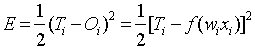By various techniques the error is then fed back through the network. Using this information, the algorithm adjusts the weights of each connection in order to reduce the value of the error function by some small amount. After repeating this process for a sufficiently large number of training cycles the network will usually converge to some state where the error of the calculations is small. In this case one says that the network has learned a certain target function. To adjust weights properly one applies a general method for non-linear optimization that is called gradient descent. For this, the derivative of the error function with respect to the network weights is calculated and the weights are then changed such that the error decreases[18].

The gradient descent back-propagation learning algorithm is based on minimizing the mean square error. An alternate approach to gradient descent is the exponentiated gradient descent algorithm which minimizes the relative entropy[19].

2.2. GMDH Neural Network

By means of GMDH algorithm a model can be represented as sets of neurons in which different pairs of them in each layer are connected through a quadratic polynomial and thus produce new neurons in the next layer. Such representation can be used in modeling to map inputs to outputs[1,2, 12]. 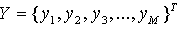The formal definition of the identification problem is to find a function so that can be approximately used instead of actual one, , in order to predict output for a given input vector as close as possible to its actual output [22]. Therefore, given M observation of multi-input-single-output data pairs so that

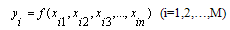it is now possible to train a GMDH-type neural network to predict the output values for any given input vector , that is

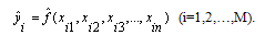The problem is now to determine a GMDH-type neural network so that the square of difference between the actual output and the predicted one is minimized, that is

.

General connection between inputs and output variables can be expressed by a complicated discrete form of the Volterra functional series in the form of

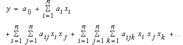(2)

which is known as the Kolmogorov-Gabor polynomial[1, 2,4,12]. This full form of mathematical description can be represented by a system of partial quadratic polynomials consisting of only two variables (neurons) in the form of

(3)

In this way, such partial quadratic description is recursively used in a network of connected neurons to build the general mathematical relation of inputs and output variables given in equation (2). The coefficient in equation (3) are calculated using regression techniques so that the difference between actual output, y, and the calculated one, , for each pair of , as input variables is minimized. Indeed, it can be seen that a tree of polynomials is constructed using the quadratic form given in equation (3) whose coefficients are obtained in a least-squares sense. In this way, the coefficients of each quadratic function are obtained to optimally fit the output in the whole set of input-output data pair, that is[16]

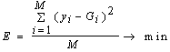(4)

In the basic form of the GMDH algorithm, all the possibilities of two independent variables out of total n input variables are taken in order to construct the regression polynomial in the form of equation (3) that best fits the dependent observations (, i=1, 2, …, M) in a least-squares sense. Consequently, neurons will be built up in the first hidden layer of the feed forward network from the observations { (i=1, 2,… M)} for different . In other words, it is now possible to construct M data triples { (i=1, 2,…, M)} from observation using such in the form

.

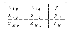Using the quadratic sub-expression in the form of equation (3) for each row of M data triples, the following matrix equation can be readily obtained as

where is the vector of unknown coefficients of the quadratic polynomial in equation (3)

(5)

and is the vector of output’s value from observation. It can be readily seen that

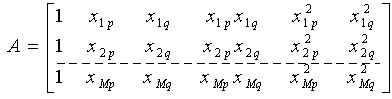The least-squares technique from multiple-regression analysis leads to the solution of the normal equations in the form of

(6)

which determines the vector of the best coefficients of the quadratic equation (3) for the whole set of M data triples. It should be noted that this procedure is repeated for each neuron of the next hidden layer according to the connectivity topology of the network. However, such a solution directly from normal equations is rather susceptible to round off errors and, more importantly, to the singularity of these equations[1,2,4,21,22].

3. Technical Indicators Used for the Study

3.1. Simple Moving Average (SMA)

This is perhaps the oldest and the most widely used technical indicator. It shows the average value of price over time. A simple moving average with the time period n is calculated by:

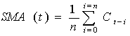where C_t is a price at time t[17]. The shorter the time period, the more reactionary a moving average becomes. A typical short term moving average ranges from 5 to 25 days, an intermediate-term from 5 to 100, and long-term 100 to 250 days. In our experiment, the window of the time interval n is 5.

3.2. Exponential Moving Average (EMA)

An exponential moving average gives more weight to recent prices, and is calculated by applying a percentage of today's closing price to yesterday's moving average. The equation for n time period is[17]:

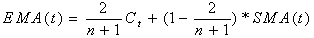The longer the period of the exponential moving average, the less total weight is applied to the most recent price. The advantage to an exponential average is its ability to pick up on price changes more. In our experiment, the window of the time interval n is 5.

4. Empirical Results

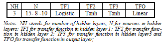
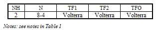
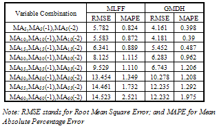
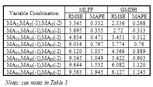
As input variables to the neural networks, we use price time series covering 01/01/2004-13/7/2009 period separately, with 2 lags of the 5-day [MA₅, MA₅(-1), MA₅(-2)], 10-day [MA₁₀, MA₁₀(-1), MA₁₀(-2)], 15-day [MA₁₅, MA₁₅(-1), MA₁₅(-2)], 30-day [MA₃₀, MA₃₀(-1), MA₃₀(-2)], 35-day [MA₃₅, MA₃₅(-1), MA₃₅(-2)], 50-day [MA₅₀, MA₅₀(-1), MA₅₀(-2)], 55-day [MA₅₅, MA₅₅(-1), MA₅₅(-2)] and 60-day [MA₆₀, MA₆₀(-1), MA₆₀(-2)] moving average crossover. 5, 10 and 15-day simple moving average and EMA are used to measure the short-term dependency, 30,35 and 40-day moving average for intermediate-term dependency and 50, 55 and 60-day moving average are used to measure the long-term dependency in gas price.

Training set is determined to include about 50% of the data set and the 25% will be used for testing and 25% for validating purposes.

During the designing of MLFF model we have changed the number of layers and neurons. Finally we found the best network in this research as a network with 3 hidden layers and 15-8-10 neurons. Almost 100 transfer function has been used and sigmoid is used for the input function and the linear function is used for output. Table 1 summarizes the characteristics of the best network.

Table 1. MLFF network characteristics

The same way, the GMDH neural network model characteristics is summarized in Table 2.

Table 2. GMDH network characteristics

Table 3 shows error rates on the testing data of the best architecture for each variables combination with simple moving average calculation.

Table 3. MLFF & GMDH network results with SMA

Table 4 shows error rates of the best architecture for each variables combination with exponential moving average calculation.

These tables suggest that the GMDH network with 3 hidden layers is a better architecture. It is also revealed that exponential moving average (EMA) has a better response for the gas price time series in this period. The result of the neural network accuracy measure (RMSE) is noticeably decreased with short-term moving like 5 and 10. This confirms the fact there is short-term dependence in gas price.

This research has been done with a Matlab's neural network toolbox that is designed based on GEovM. We have changed some part of its code to be more flexible and dynamic.

Table 4. MLFF & GMDH network results with EMA

5. Conclusions

Gas is an important traded commodity and forecasting its price, has important implications economically. Despite the significant number of studies on gas and its price, the precise pricing mechanism in the gas market has not been deciphered. Many of them are based on neural network and it shows they are much better than the other methods. This paper used two types of neural networks to investigate the price of gas. It has been shown that GMDH type neural networks have better results when the associated system is so complex and the underline processes or relationship are not completely understandable or display chaotic properties.

We have used gas price time series and its moving average as the input to the neural network and the results show:

1- The GMDH has better response relative to MLFF neural network.

2- Gas price has short-term dependence to its history.

3- The exponential moving average is a better choice relative to simple moving average, if the moving average techniques are used.

Notes

¹GEovM is a software package that has been designed by the University of Gilan