Sreejata Dutta1, Soham Ghosh2
1Department of Biostatistics & Data Science, University of Kansas, Kansas City, USA
2School of Engineering, University of Kansas, Overland Park, USA
Correspondence to: Sreejata Dutta, Department of Biostatistics & Data Science, University of Kansas, Kansas City, USA.
| Email: |  |
Copyright © 2021 The Author(s). Published by Scientific & Academic Publishing.
This work is licensed under the Creative Commons Attribution International License (CC BY).
http://creativecommons.org/licenses/by/4.0/

Abstract
With the increasing demand for electrical energy worldwide and the proportionate inflation of natural resources, it is important to predict the electrical power output from baseload combined cycle power plants and the factors affecting the yield per hour. Finding reliable factors not only improves the performance of the power plant in terms of production or distribution but also ensures the proper utilization of natural resources (or fuels) with minimal effect on the environment and effective cost management. Though there are sophisticated machine learning models for predicting full load electrical power output, often these deployed models are unable to draw inferences. Thermodynamic models on the other hand are oftentimes too complex, are valid only under a set of assumptions, and are generally non-linear in nature adding to the computation time. Keeping these limitations in mind, the objectives of this study are to find potential predictor variables that affect the power output yield per hour and then use these inferences to construct a simple yet effective model to predict the electrical power output in combined cycle power plants. The dataset used for this study is from a combined cycle power plant over a span of six years (2006-2011), with the power plant operating in a full load. A combined cycle power plant is composed of gas turbines, steam turbines, and heat recovery steam generators. The gas and steam turbines generate the electricity which is combined in one cycle and is transferred from one turbine to another. The input features of the dataset considered for this study consist of average ambient variables: ambient temperature, ambient pressure, relative humidity, and exhaust vacuum which are used to predict the average hourly electrical power output.
Keywords:
Combined cycle power plant, Linear modelling, Regression, Power generation, Statistical inference, Prediction
Cite this paper: Sreejata Dutta, Soham Ghosh, Predicting Electrical Power Output in a Combined Cycle Power Plant - A Statistical Approach, International Journal of Energy Engineering, Vol. 11 No. 2, 2021, pp. 17-26. doi: 10.5923/j.ijee.20211102.01.
1. Introduction
Steam turbines systems generate most of the electrical power generated worldwide. The prediction of the real power output of such baseload plants is important for the effective operation of the electric grid, especially in countries where the electric grid is still developing, and natural resources are in limited quantities. Gas turbine power output mainly depends on the ambient parameters such as ambient temperature, atmospheric pressure, and relative humidity whereas steam turbine power output has a direct relationship with the vacuum at the exhaust. [1,2,3]. Gas turbine derivatives, such as combined cycle power plants (CCPP) are being established all over the world to fulfill the demand for electrical energy considering both economic and environmental concerns. It has been found that the three ambient predictor variables: ambient temperature (AT), ambient pressure (AP), and relative humidity (RH) affects while exhaust vacuum (V) affects the production of steam turbines.Hence, the objective of this paper is to study the association of the average ambient variables with the hourly yield of electrical power output and find out reliable predictors for CCPP that would help inefficient production. This in turn would help in the proper utilization of resources in terms of maximum yield and minimum cost of production.The main motivation for this study is that there exist thermodynamical studies to predict the output of a CCPP. However, detailed analysis of a system by using thermodynamical approaches [5,6] is a computationally intense effort, and sometimes the result of such analysis might be inaccurate due to the interaction of several assumptions being considered and the nonlinear nature of the governing equations. On the other hand, machine learning models have gained steam in recent years [7,8,9]. The inability to draw inferences from these wide-scale sophisticated state-of-the-art models remains a concern.To overcome these obstacles, the analysis here is undertaken using a statistical approach of first drawing an inference from the data about the potential predictors, and then using the inferences a predictive model would be constructed for predicting the output of a thermodynamic system, which is a CCPP with two gas turbines, one steam turbine, and two heating systems in full load. The remainder of the paper is organized as follows: section 2 highlights the statistical methods used in this study along with a description of the data source and general model assumptions. Section 3 presents a preliminary analysis of the potential predictors and a brief summary of the response variable. Section 4 throws light on the multicollinearity between the different predictor variables and explores the model selection and validation. Section 5 presents an overview of the goodness of fit test. Section 6 present a discussion of the statistical findings of the study, before ending with a concluding remark in section 7.
2. Statistical Methods
The primary objective of this study is to investigate the potential predictors, that is the average ambient variables, that affect the electrical power output in a CCPP; which would then be used to predict the electrical power output.
2.1. Material and Methods: Data Source
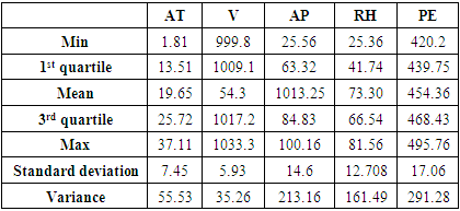
The dataset was obtained online in Microsoft excel format [10].The dataset was collected over a period of six years (2006 - 2011) from a combined cycle power plant when the plant was set to operate on full load. A sample size n = 9568 was collected and shuffled five times; the data generated from each of these shuffles was provided in separate spreadsheets. For each shuffling 2-fold cross-validation (CV) [11] was carried out and the resulting ten measurements are used for statistical testing. For data analysis, only one of the spreadsheets is considered among the collection of five spreadsheets. The dataset consists of hourly average ambient variables per second taken from various sensors located around the plant. Variables in the data set include ambient temperature (AT) ranging from 1.81°C to 37.11°C, ambient pressure (AP) ranges from 992.89 − 1033.30 millibar, relative humidity (RH) in the range 25.56% to 100.16%, exhaust vacuum (V) range from 25.36 − 81.56 cm Hg and net hourly electrical energy output (PE) 420.26 − 495.76 MW.
2.2. Material and Methods: Statistical Analysis
The data analysis is conducted using the statistical software R version 3.5.2 (2018-12-20) and the study focuses mainly on multiple linear regression. A significance value (α) = 0.05 is considered in this study. The input features are continuous variables, which are summarized using the five summary statistics (mean, median, minimum, maximum, and standard deviation). The original dataset is divided into 90:10 training - testing sets. Each of the predictor variables is explored individually and the preliminary investigation is conducted on the training dataset. No missing values were found in the dataset. The automatic model selection method has been used on the training set to arrive at the final model. The final model is validated using model diagnostics and the goodness of fit tests. The model assumptions including homoskedasticity, normality, and independence of error terms, as well as linearity of the association between the outcome and the ambient variables, are checked before finalizing the estimated fitted regression function. The finalized model is then used on the test set to find the predicted values and compared to the observed value at a 95% prediction interval.
3. Preliminary Data Analysis
Preliminary data analysis help in detecting skewness, presence of outliers or can also suggest if transformations are necessary to fit a better model. Preliminary data analysis also gives an idea about the association of the potential predictors with the outcome.
3.1. Analysis of the Potential Predictors
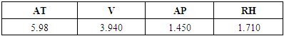
Figure 1 illustrates the distribution while Table 1 presents the summary statistics of the individual ambient variables: ambient temperature (AT), ambient pressure (AP), relative humidity (RH), and exhaust vacuum (V). Figure 1 (a), (b), and (d) shows that ambient temperature (AT), ambient pressure (AP), and exhaust vacuum (V) appear to be approximately symmetrical while Figure 1 (c) shows relative humidity (RH) to be a little skewed (left or negatively skewed). Some outliers can also be detected in ambient pressure (AP) and relative humidity (RH) (Figure 1 (b) and (c)). 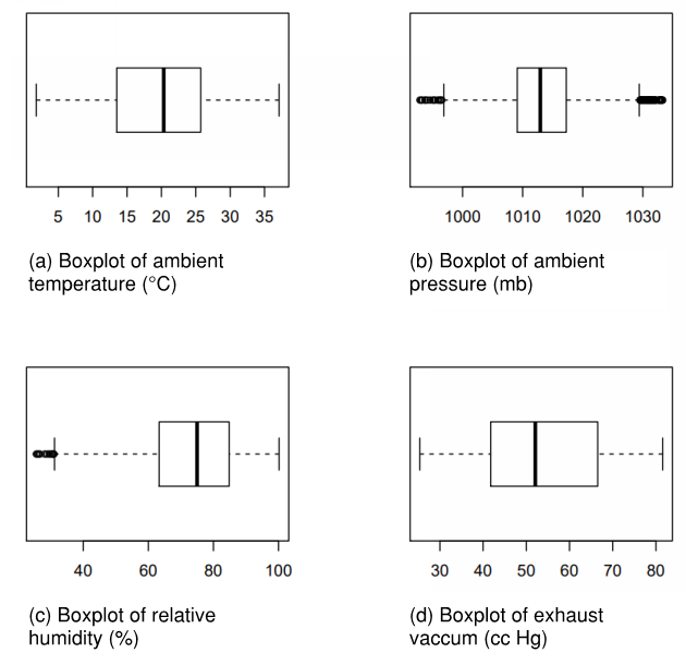 | Figure 1. Analysis of predictors using box and whisker plots |
3.2. Analysis of the Electrical Power Output
Preliminary data analysis on the electrical power output (PE) shows that the response variable is positively skewed as the whiskers to the right are longer than the ones on the left. The presence of outlying values is not observed in Figure 2. The summary statistics of PE have been presented in Table 1.Table 1. Basic statistics for dataset variables
 |
| |
|
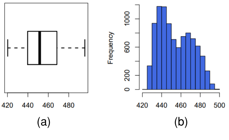 | Figure 2. Distribution of electrical power output through (a) box and whisker plot, (b) histogram |
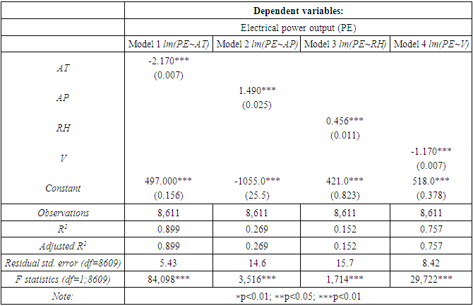
3.3. Effect of Ambient Temperature (AT) on the Electrical Power Output (PE)
Figure 3 illustrates the scatter plot for the ambient temperature (AT) and electrical power output (PE) with the fitted regression line. The resultant predictive model can be written as (1), where  represents the electrical power output (PE) and
  is the ambient temperature (AT). The model states that for every 1°C rise in ambient temperature (AT), the electrical power output (PE) drops by 2.171 MW per hour.
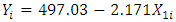 | (1) |
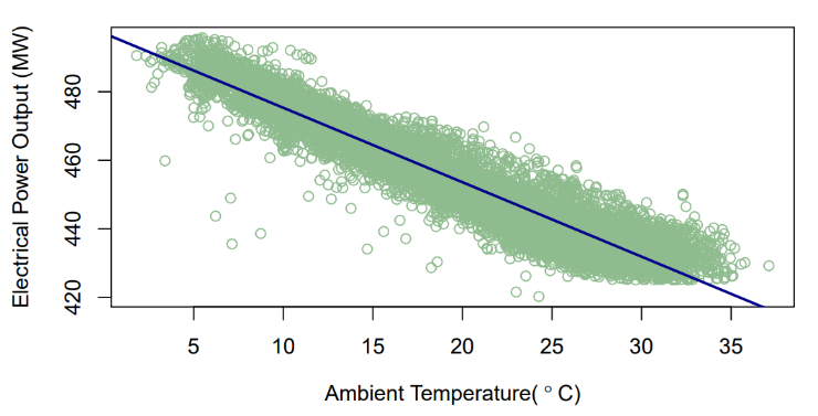 | Figure 3. Prediction of PE (MW) with reference to AT (°C) |
3.4. Effect of Ambient Pressure (AP) on the Electrical Power Output (PE)
Figure 4 illustrates the scatter plot for the ambient pressure (AP) and electrical power output (PE) with the fitted regression line. The resultant predictive model can be shown as (2), where  represents the electrical power output (PE) and
  is the ambient pressure (AP).
 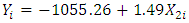 | (2) |
The model states that for every 1 mb (or millibar) rise in ambient pressure (AP), the electrical power output (PE) increases by 1.49 MW per hour.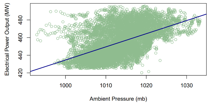 | Figure 4. Prediction of PE (MW) with reference to AP (mb) |
3.5. Effect of Relative Humidity (RH) on the Electrical Power Output (PE)
The scatter plot of relative humidity (RH) and electrical power output (PE) is illustrated in Figure 5 with the fitted regression model. Thus, the resultant predictive model is represented by (3), where  represents the electrical power output (PE) and
  is the relative humidity (RH). It can thus be inferred that for every one percent rise in relative humidity (RH) increases the electrical power output by 0.456 MW per hour.
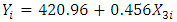 | (3) |
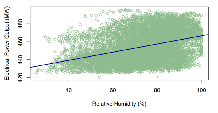 | Figure 5. Prediction of PE (MW) with reference to RH (%) |
3.6. Effect of Exhaust Vacuum (V) on the Electrical Power Output (PE)
Figure 6 illustrates the scatter diagram of exhaust vacuum (V) and electrical power output (PE) produced after fitting the linear regression model. The resultant predictive model can be represented by (4), where  represents the electrical power output (PE) and
  is the exhaust vacuum (V). The predictive model can thus infer that for every 1 cm Hg rise in exhaust vacuum, the electrical power output decreases by 1.168 MW per hour.
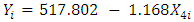 | (4) |
 | Figure 6. Prediction of PE (MW) with reference to V (cm Hg) |
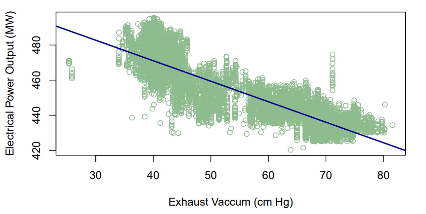
Table 2 shows the summary statistics for each the fitted regression model (1), (2), (3), and (4) along with the model fit statistics: coefficient of determination (R2), F statistics, adjusted  and MSE is in Table 2.
Table 2. Summary statistics of four separate models: outcome and each of the predictors
 |
| |
|
4. Multicollinearity, Model Selection and Validation
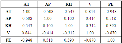
In a typical scenario, multicollinearity [12] makes data analysis complicated. The association between predictors is often observed by considering the coefficient of correlation or Pearson correlation (r). Values of r closer to ±1 indicate that the predictors are highly correlated. Figure 7 and Table 3 show the correlation matrix or pairwise Pearson’s correlation coefficients. The r values between the electrical power output (PE) and all the ambient variables are greater than ±5, except relative humidity (RH). The r value between ambient temperature (AT) and exhaust vacuum (V) seems to be high (0.84). Once the model has been finalized, the effect of multicollinearity on the final model fit can be analyzed using the variation inflation factor (VIF) [13]. In case the values of VIF exceed 10, it is often regarded as the presence of multicollinearity and measures need to be taken.Table 3. Correlation matrix for the dataset
 |
| |
|
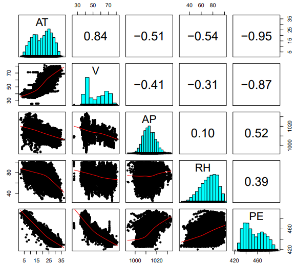 | Figure 7. Pairwise Pearson’s correlations coefficients for the ambient variables |
4.1. Model Selection: Automatic Variable Selection Method
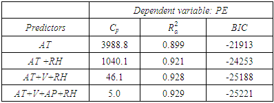
The automatic variable selection method is a starting point to eliminate the redundant variables from the model. The “regsubsets” function from the “leap” package in R is used. The best model is selected based on Mallow’s Cp, BIC, and  [15,16]. The automatic variable selection method selects the model which has the least value for Mallow’s Cp and BIC, while the model with the largest value of
  is considered best. For this particular data set, the best model includes all four ambient variables. Refer to Table 4 for a summary of the automatic selection method.
Table 4. Automatic selection method statistics
 |
| |
|
Thus, the final model can be expressed as (5).  | (5) |
where,  is the electrical power output
 is the ambient temperature
 is the exhaust vacuum
 is the ambient pressure
 is the relative humidity
 is the error term;
  i = 1,2,3 …, 8611
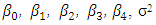 are the unknown parameters to be estimated which is discussed in section 6. However, the model assumptions must be checked and validated before diving into the model parameter estimates. Thus, the remainder of this section is dedicated to model validation and diagnostics.
4.2. Model Validation
4.2.1. Added Variable Plots (Residual Plots)
The added variable, also known as partial residual plots, are useful to detect the significance of a particular variable in the presence of the other covariates. It can also be useful in detecting outliers or in case any transformations are required in the model predictors [15]. Figure 8 represents the partial residual plot suggesting that no transformations are required in the current model. However, the presence of outliers is detected.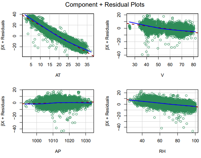 | Figure 8. Added variable plots (showing component and residual plots) |
4.2.2. Outliers and Influential Points
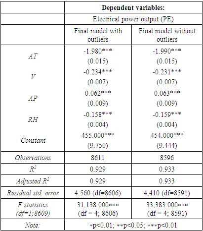
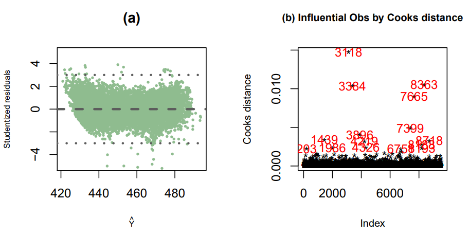
To detect outliers in this study, a studentized residual plot and cook’s distance are considered. For a more rigorous treatment of Cooks distance, including a modification of the classical form in the context of regression models, readers are encouraged to refer [14]. As per standards, 99% of the data points should be within the range of ±3 [15] which is confirmed by Figure 9 (a). Fifteen outliers are detected in the study as evident from Figure 9 (b). To check if these outliers are influential to the model fit, a linear model is considered excluding these data points. It is found that the final model is robust to these data points since no significant changes in model statistics are observed (Table 5), hence these fifteen observations are included in the final model. Table 5. Comparison of model summary with and without outliers
 |
| |
|
 | Figure 9. Detecting outliers using studentized residuals and Cook’s distance |
4.3. Model Diagnostics
Figure 10 shows that all the model assumptions are satisfied. Figure 10 (a) shows that the model follows homoskedasticity or equal variance. Figures 10 (b) and (c) confirm that the error terms follow normality. The independence of error terms is also quite evident in the sequence plot (Figure 10 (d)). However, since the dataset was shuffled, assessing the independence might not be technically possible. 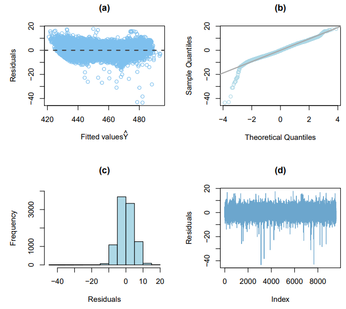 | Figure 10. Residual’s diagnostics showing a. fitted values, b. theoretical quantiles, c. residuals, and d. index |
Since the model is finalized and the assumptions are validated, multicollinearity is assessed using the VIF. Table 6 shows the VIF values exhibited by the final model, which are significantly less than 10. Thus, it can be assumed that multicollinearity is not significant in the finalized model (5).Table 6. Variation inflation factor (VIF) values from the final model
 |
| |
|
5. Goodness of Fit Test and Results
For each of the ambient variables, we test if there exists a linear association with power output (PE) using a two-tailed t-test individually. Since more than one t-test is conducted, Bonferroni’s multiple comparisons is considered [15]. The t-test considers the following hypothesis:* Null hypothesis:  * Alternative hypothesis:
  The decision is taken considering
  where,-t* is the test-statistics for the t-test
 is the observed slope coefficient
 is the expected slope coefficient of the fitted regression model
 is the sampling variability of
  The t* is tested against
  where, -α is the level of significance = 0.05-df is the degrees of freedom, i.e., df = number of observations minus number of estimate parameters = (n − 2)If
  H0 is rejected else the decision is taken in the favour of H0. The decision rule also considers the p-value and the R2. If, p-value ≤ α, the decision is to reject H0 else we fail to reject H0 [15].While considering the coefficient of determination (R2), if the value is closer to 1, the association is considered strong as the percentage or proportion of explained variation in electrical power output (PE) is significantly higher than the unexplained variation. However, if R2 is closer to 0, the model will be not be considered as a good fit as it would indicate that there exists no or a weak association between the ambient variables and electrical power output (PE) as the percentage of unexplained variation is significantly low).
5.1. Effect of Ambient Temperature (AT) on the Electrical Power Output (PE)
The t-test rejects  thus, concluding that there exists evidence of a linear association between ambient temperature (AT) and electrical power output (PE). The R2 explains that model (1) can explain 89.9% of the unexplained variation in electrical power output (PE), indicating that the model is a good fit.
5.2. Effect of Ambient Pressure (AP) on the Electrical Power Output (PE)
The t-test rejects  and concludes that there exists evidence of a linear association between ambient pressure (AP) and electrical power output (PE). The R2 for model (2) is only 26.9%, which indicates that ambient pressure (AP) is not strongly associated with electrical power output (PE).
5.3. Effect of Relative Humidity (RH) on the Electrical Power Output (PE)
The t-test  rejects the H0. Though there exists sufficient evidence of a linear association between relative humidity (RH) and electrical power output (PE), the value of R2 is relatively small. Only 15.2% of the unexplained variation can be explained by the fitted model (3) while the other 84.4% remains as unexplained variation in PE.
5.4. Effect of Exhaust Vacuum (V) on the Electrical Power Output (PE)
The t-test reject the  suggesting that a linear association exists between exhaust vacuum (V) and electrical power output (PE). The percentage of explained variation is high for model (4). Around 75.7% of the unexplained variation in electrical power output (PE) is explained (4) while only 24.3% remains as the unexplained variation.
5.5. Discussion of Results from the T-Test
The results from the t-test show that a linear association exists between PE and all the average ambient variables (AT, AP, RH, and V). To find the most effective predictor variable, the R2 or  can be referred to, which indicates the percentage or proportion of explained variation in electrical power output (PE) to the total variation in electrical power output (PE). Referring to the R2 and
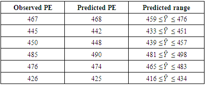
  (Table 2) value, variables that can predict the maximum percentage of unexplained variation are the ambient temperature (AT), followed by exhaust vacuum (V) while the variable that explains the least of the unexplained variation in PE is relative humidity (RH). To confirm that ambient variables can significantly predict the electrical power output (PE), the predicted values are compared to the actual observed values from the test set (Table 7). At 95% prediction interval, it is found that the model performs well in estimating the average power electrical output using ambient variables.
Table 7. Validating model prediction
 |
| |
|
6. Discussion
The model estimates from (5) can be summarized as below:  | (6) |
where, Yi is the electrical power outputX1i is the ambient temperatureX2i is the exhaust vacuumX3i is the ambient pressureX4i is the relative humidity is the error term;
 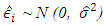 i = 1,2,3 …, 8611The study shows that the average ambient variables: ambient temperature (AT), ambient pressure (AP), relative humidity (RH), and exhaust vacuum (V) can predict the electrical power output (PE) per hour in a combined cycle power plant (CCPP) having both gas and steam turbines. The average ambient variables were explored individually, and the two-tailed t-test was conducted on each of the fitted linear regression models and a linear association was found in each case. The final model (6) was able to explain about 92.9% of the unexplained variation in the electrical power output (PE), indicated by both R2 and
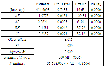
  (Table 8). Further, model validation and residual analysis confirmed the model assumptions. The estimated mean squared error (MSE) or
  from the final model is 20.8.
 Table 8. Statistics table for the regression model
 |
| |
|
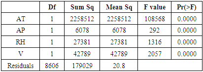
Table 8 shows the estimated regression coefficient, the standard error, t value, p-value associated with each of the predictors,  MSE and F-statistics of the final model. Table 9 shows the ANOVA table for the final model Exploring the test statistics, it is found that the strongest association among all average ambient variables and power output is best explained by the linear association of ambient temperature and exhaust vacuum, which is evident by the fact that about 90% and 76% of the unexplained variation in the output power per hour (Table 2) and also by the magnitude of the
  corresponding to ambient temperature and exhaust vacuum.
Table 9. ANOVA table for the regression model
 |
| |
|
The study showed that except for ambient pressure all the other predictors exhibit a negative association with the response variable electrical power. Given the well-behaved residuals and high percentage of explained variation of 92.9% 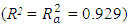 (Table 8), it can be concluded that the model performs well.At 95% prediction interval, the electrical power output from the predicted model was compared with the observed values and it confirmed that ambient variables can be used to predict the electrical power output in a CCPP operated by both gas and steam turbines (Table 7). The presence of outliers was detected in the model and it was found that the model is robust to outliers (Table 5).
7. Conclusions
This paper presents a statistical model for a prediction of the electrical power output of a baseload operated CCPP when it was full load. Instead of thermodynamical modeling which involves a substantial number of assumptions and nonlinear system equations, or black-box machine learning models with multiple neural networks with unknown weights and biases, a statistical approach was used which can not only predict but draw useful inferences. Substantiated with large sample size and absence of missing values, this study’s strength lies in less sampling variability thus ensuring better prediction, which is evident by the model’s robustness to the outliers. The two main purposes of this study were to discover the predictors which potentially have a linear association with full load electrical power output, and if these potential predictors could accurately predict the full load power output. Both of these objectives were achieved using multiple linear regression models. Future work may be undertaken to refine the input to this predictive model by first predicting the next day’s ambient variables more precisely and investigating the prediction of electrical power output for different types of power plants. Further, given that the ambient temperature was essentially found to be the most influential variable, more studies can be conducted on the effect of temperature on different types of power plants and how the temperature variance throughout the day affects the power output. Another interesting approach can involve testing the association of electrical power output with the relative humidity and ambient pressure since this study was not able to capture a strong association of the power output with these two ambient variables.
References
| [1] | S. H. Ali, A. T. Bahetaa and S. Hassan, "Effect of Low-Pressure End Conditions on Steam Power Plant Performance," in ICPER 2014 - 4th International Conference on Production, Energy, and Reliability, Perak, Malaysia, 2014. |
| [2] | P. Hundi and R. Shahsavari, "Comparative studies among machine learning models for performance estimation and health monitoring of thermal power plants," Applied Energy, vol. 265, 2020. |
| [3] | I. S. Rout, A. Gaikwad, V. K. Verma, and M. Tariq, "Thermal Analysis of Steam Turbine Power Plants," Journal of Mechanical and Civil Engineering, vol. 7, no. 2, pp. 28-36, 2013. |
| [4] | Cast-Safety, "Fundamentals of Gas Turbine Engines," 2010. [Online]. Available: https://www.cast-safety.org/pdf/3_engine_fundamentals.pdf. [Accessed 10 2021]. |
| [5] | A. Ganjehkaviri, M. N. Mohd Jaafar, P. Ahmadi, and H. Barzegaravval, "Modelling and Optimization of Combined Cycle Power Plant Based on Exergoeconomic and Environmental Analyses," Applied Thermal Engineering, vol. 67, no. 1-2, pp. 566-578, 2014. |
| [6] | I. K. Thamir and M. N. Mohammed, "Thermodynamic Evaluation of the Performance of a Combined Cycle Power Plant," International Journal of Energy Science and Engineering, vol. 1, no. 11, 2015. |
| [7] | P. Tüfekci, "Prediction of Full Load Electrical Power Output of a Base Load Operated Combined Cycle Power Plant Using Machine Learning methods," International Journal of Electrical Power & Energy Systems, vol. 60, pp. 126-140, 2014. |
| [8] | L. Ivan, A. Nikola, V. Mrzljak and Z. Car, "Genetic Algorithm Approach to Design of Multi-Layer Perceptron for Combined Cycle Power Plant Electrical Power Output Estimation," Energies, vol. 12, no. 22, 2019. |
| [9] | Z. Qu, J. Xu., Z. Wang, R. Chi, and H. Liu, "Prediction of Electricity Generation from a Combined Cycle Power Plant Based on a Stacking Ensemble and its Hyperparameter Optimization with a grid-search method," Energy, vol. 227, 2021. |
| [10] | P. Tüfekci, "Combined Cycle Power Plant Data Set," University of California: Machine Learning Repository, 2014. |
| [11] | M. W. Browne, "Cross-Validation Methods," Journal of Mathematical Psychology, vol. 44, no. 1, pp. 108-132, 2000. |
| [12] | A. Alin, Multicollinearity, Wiley Interdisciplinary Reviews: Computational Statistics, 2010. |
| [13] | M. O. Akinwande, H. G. Dikko, and A. Samson, "Variance Inflation Factor: As a Condition for the Inclusion of Suppressor Variable(s) in Regression Analysis," Open Journal of Statistics, vol. 5, no. 7, 2015. |
| [14] | J. A. Dı́az-Garcı́a and G. González-Farı́as, "A note on the Cook's distance," Journal of Statistical Planning and Inference, vol. 120, no. 1-2, pp. 119-136, 2004. |
| [15] | M. H. Kutner, C. J. Nachtsheim, J. Neter and W. Li, Applied Linear Statistical Models, 5th ed, McGraw-Hill, 2014. |
| [16] | O. Darnius and G. Tarigan, "Simulation Method of Model Selection Based on Mallows' Cp Criteria in Linear Regression," Journal of Physics: Conference Series, vol. 1116, no. 2, 2018. |

 Abstract
 Reference
 Full-Text PDF
 Full-text HTML