Nkontchou Ngongang François1, Tchawe Tchawe Moukam1, Tientcheu Nsiewe Max-well2, Djiako Thomas3, Djeumako Bonaventure1, Tcheukam-Toko Dénis4
1Department of Mechanical Engineering, ENSAI, University of Ngaoundere, Cameroon
2Department of Fundamental Sciences, EGCIM, University of Ngaoundere, Cameroon
3Department of Mechanical Engineering and Energy, ISTA, University Institute of the Gulf of Guinea, Cameroon
4Department of Mechanical Engineering, COT, University of Buea, Cameroon
Correspondence to: Tchawe Tchawe Moukam, Department of Mechanical Engineering, ENSAI, University of Ngaoundere, Cameroon.
| Email: |  |
Copyright © 2021 The Author(s). Published by Scientific & Academic Publishing.
This work is licensed under the Creative Commons Attribution International License (CC BY).
http://creativecommons.org/licenses/by/4.0/

Abstract
This work deals with determining the characteristics of the flow through the penstock of the Three Gorges dam in China. It also allows us to understand the influence of the diameter of the water duct on the modification of the flow structure in the penstock. To achieve our goals, the Eulerian resolution of the Navier-Stokes equations is done by a RANS approach using the FLUENT calculation code. The turbulence model applied is that with two k-ɛ equations. The results show constant velocities upstream of the dam until approaching the water intake at a distance of about 15m upstream, keeping an asymmetric shape in the different sections constituting the penstock. The maximum velocities are observed on the innerside of the various elbow. Layers of positive pressure are also visible in the penstock away from the walls; suggesting substantially coaxial and positive iso-pressures in high velocity zones, with a maximum directed towards the center of the penstock. This phenomenon thus goes against the high velocity-low pressure hypothesis, and may be justified by the geographical arrangement of the penstock, associated with its large diameter.
Keywords:
Hydroelectric dam, Penstock, Dynamic fields, CFD
Cite this paper: Nkontchou Ngongang François, Tchawe Tchawe Moukam, Tientcheu Nsiewe Max-well, Djiako Thomas, Djeumako Bonaventure, Tcheukam-Toko Dénis, Determination of the Dynamic Field in the Penstock of the Trois-Gorges Dam by a Numerical Approach, International Journal of Energy Engineering, Vol. 11 No. 1, 2021, pp. 9-16. doi: 10.5923/j.ijee.20211101.02.
1. Introduction
The production of electrical energy by hydroelectric power stations is booming around the world. Of the equipment constituting these structure, the penstock and the turbine constitute sensitive equipment because of their impact on the performance of the entire structure [1]. They are at the origin of more than half of the studies carried out on these master piece according to our research.This work focuses on penstocks that channel pressurized water to the turbine. They can be mild steel, glass reinforced plastic (GRP), reinforced concrete (RC), wooden staves, cast iron and high density polyethylene (HDPE), etc. However, due to greater applicability and availability, mild steel is the most widely used [2]. For less expensive and rapid studies, researchers use a modern tool that facilitates studies in the field of fluid mechanics.The CFD for "Computational Fluid Dynamics" allows the study of complex flows encountered in engineering. Its development, with the digital age, now results in enormous possibilities so that it is possible to model the three-dimensional flow [3]. In addition, it offers the possibility of taking an in-depth look at the flow, which helps in understanding complex phenomena. These phenomena may be different depending on the shape of the penstock, or another parameter such as the shape of the water intake.In this document, we will present studies carried out on the penstock of the Three Gorges dam in China. The main objective in this first document relates to the determination of the hydraulic characteristics observed on the flow through the penstock of this dam. Thus, we will present cross sections of the penstock at very precise distances, in order to observe the fluid layers crossing the penstock to the turbine inlet.
2. Material and Methods
2.1. Assumption of Calculation Domain
The model of our penstock is shown in Figure 1 below for a maximum flow rate of 970 m3/s. The structure is made up of three pipe sections linked together by elbows:• The first section is located between the water intake and the first elbow;• The second section is the part which is found between the two elbows;• The third section is the one between the second elbow and the turbine inlet.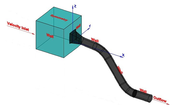 | Figure 1. Three-dimensional model with boundary condition |
The turbulence model used is k-ε Realizable because it is well suited to boundary layers with a strong adverse pressure gradient, to strong curvature and vortex flows and a considered isotropic. The second order equations are solved with the velocity-pressure coupling method SIMPLEC and a convergence criterion of 10-6. The function near walls function considered is the standard wall function, and the discretization scheme is Body Force Weighted. The approach flow is stationary and the turbulence is isotropic.
2.2. Governing Equations
The flow is incompressible and isothermal with constant viscosity, and can be described by the velocity and pressure field governed by the Navier-Stokes equations [4] quoted by [5]. The fluid is assumed to be a Newtonian fluid. We have:  | (1) |
The dynamic conservation is: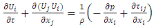 | (2) |
where  represents the velocities in
  coordinate directions;
  is the static pressure load,
  the constant density, and
  the viscous stress tensor. For a Newtonian fluid:
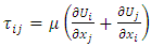 | (3) |
In the flows, the variations are too rapid to be described in time and space. Velocity details are lost. We can adopt the following decomposition for the pressure and the velocity: | (4) |
where  and
and  are the average components of the fluctuating velocity
  . In the same way for the pressure and the other scalar values:
 | (5) |
Where  represents a scalar such as pressure, energy, or other concentration.Substituting expressions of this form for the flow variables in the instantaneous continuity and momentum equations while taking a time average, we obtain the average momentum equations. They can be written in the form of Cartesian tensor:
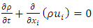 | (6) |
 | (7) |
Additional terms now appear that represent the effects of turbulence. The Reynolds stress  must be modeled to close the equation. The closing of the equation uses Boussinesq's approximation [6]:
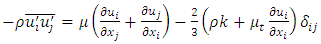 | (8) |
The model of the transport equations for k and  is:
is: | (9a) |
 | (9b) |
where: 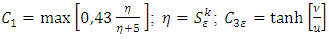
 represents the degree of influence of volume forces,
  is the component of the flow velocity parallel to the gravitational vector, and
  is the component of the flow velocity perpendicular to the gravitational vector.In these equations,
 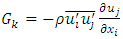 represents the generator term of the kinetic energy of turbulence due to the mean of the calculated velocity gradient,
 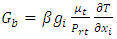 is the generator term of the kinetic energy of turbulence due to the volume forces,
  represents the fluctuation of the expansion in compressible turbulence.
  and
and  are their constants.
  et
et  are the turbulent Prandtl numbers for
  and
and  respectively [7] quoted by [1].
  and
and  are user-defined terms.The turbulent viscosity is given by:
 | (10) |
The difference between the three models is in the term of  which is given by:
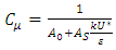 | (11) |
The constants are given by: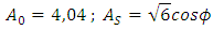

3. Results and Discussion
3.1. Mesh Geometry
Solving the equation of conservation of mass, momentum and energy equations requires the use of boundary conditions for each dependent variable. The velocity conditions at the walls and at the openings are shown in Figure 1 above. The nearing flow is always assumed to be stationary.To better understand the evolution of the flow structure in the penstock, we have divided each of the sections into three parts as we will see below. We see that the velocity is constant upstream of the dam until near the water intake, at a distance of about 15m upstream. After this distance, we see a change in the flow structure under the influence of the water intake.The legends presented on the fields correspond to the average values existing in the entire structure. As the modeling is three-dimensional, Figures 2 below show us a longitudinal section (median plane) of the mesh used in the study. We have in this figure numbers corresponding to the different portions studied.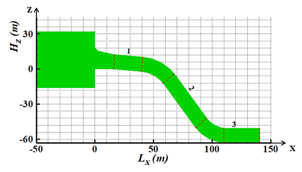 | Figure 2. Structure of the mesh with different portions studied |
We bring out in Figure 3 the mean sensitivities of the meshes corresponding to four mesh structures that have been the subject of the study in this work. | Figure 3. Mesh sensitivity |
3.2. Velocity Fields
From the study of the sensitivity of the mesh, we find that the mesh no longer has a very large impact on the profiles obtained from 223,600 cells as shown in Figure 3 above. However, we opted for the more dence mesh, of 1049946 cells.To better understand the evolution of flow layers in the pipe so we be located in relation to each section distance, a longitudinal outline of the part of the structure studied is presented. This longitudinal section corresponds to the dynamic field studied, namely the velocity field and the pressure field.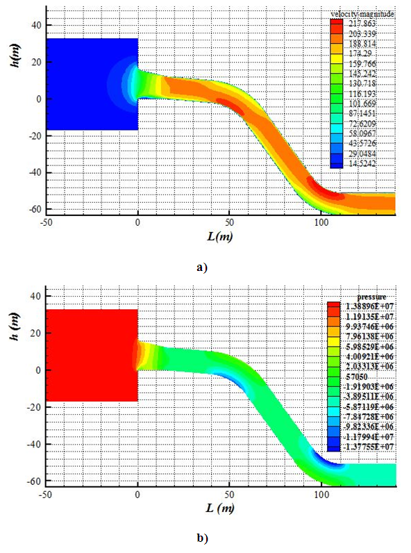 | Figure 4. Velocity (a) and pressure (b) field at y = 0 m |
The velocity increases as we approach the penstock. We then observe layers of high velocity crossing the penstock with an asymmetric shape to the axis of the pipe in different sections. The maximum velocities are on the innerside of the various curves, with a heavier layer at the second elbow.For the pressure field, the high pressure layers are observed in the upstream zone (reservoir) at the water intake. Similarly, low pressure layers are observed in the innerside of each curve. However, we also see layers of positive pressure in the penstock away from the walls. For an in-depth observation of these different phenomena, we will subsequently make cross-sections on each section of the penstock. These three transects better reflect the flow evolution in this section of the penstock. Observing Figure 5a and at the start of this portion (x = 15m), the maximum velocities are observed near the walls in separate layers; the vast majority being on the upper side. As we move forward in the pipe.Thus, we have opted to make three cuts for each section. The entrance to the water intake is located at a distance of x=0m.
3.2.1. First Section
The three cuts of this section are located at the following respective distances: x = 15 m, x = 28 m which approximately represents the middle, and x = 40 m for the exit as shown in Figures 5a and 5b below.These layers concentrate towards the center of the penstock as we can see at the distance x = 28m. At the exit of this portion (entry of the elbow), this curve has an elliptical shape, and is pressed against the bottom wall of the pipe. Note that from the fields, we seem to be in the presence of three layers in the cuts presented.Figure 5b shows the pressure field. At x = 15 m, we observe a pressure force towards the center of the pipe, thus reflecting the effect of the concentration of the intake on the inlet flow. Its quadrilateral shape represents the shape of the socket. The flow in its evolution towards the elbow presents a maximum pressure towards the center of the pipe, thus limiting the hypothesis of high pressure low velocity. 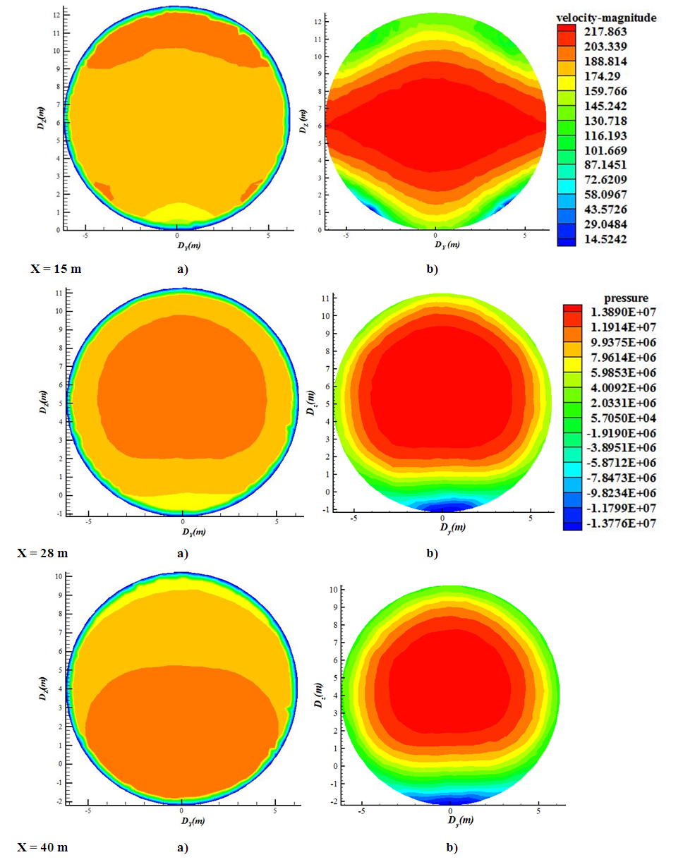 | Figure 5. Velocity (a) and pressure (b) field in section 1 |
At the exit of the first elbow, we seem to be in the presence of two layers, with the high velocity layer observed on the bottom wall as shown in figure 6a, at the distance x = 57m.We subsequently observe substantially coaxial iso-pressures with a maximum, directed towards the center of the penstock. However at the distance x = 40m, the low pressure layer is observed on the bottom wall.
3.2.2. Second Section
For this section, the three cuts are placed at the respective distances x = 57m (for the entrance), x = 70 m (for the middle) and x = 95 m (for the exit or the entry into the second elbow).Moving towards the middle of the portion, we seem to be in the presence of 3 layers, with the high velocity layer observed towards the upper part in the penstock. At x = 95m, we observe several fluid layers, with a high velocity layer practically stuck to the upper wall (ceiling) of the penstock. In figure 6b, we observe the same iso-pressure as noted previously, with the layers of high pressure in the upper part of our penstock (at x = 57m). As they move away in the section, these layers remain at the top of the penstock, keeping its ovoid shape. Once again, we observe non-zero iso-pressures in high velocity zones; which again goes against the high velocity-low pressure phenomenon.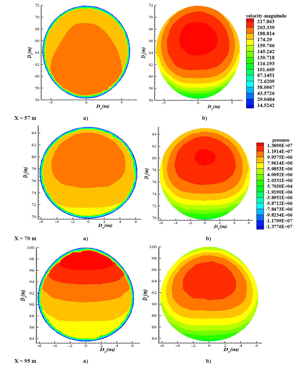 | Figure 6. Velocity (a) and pressure (b) field in section 2 |
The velocity fields present us with several fluid layers at the exit of the second elbow as we can see in figure 7a above, at x = 112m. As you approach the turbine, the flow becomes symmetrical as shown in the figure above at x = 140m.This new phenomenon can be justified by the geographical disposition of the penstock, associated with its large diameter. However, this is one of the objects of an ongoing study.
3.2.3. Third Section
As with the previous sections, the distances here are x = 112 m (for the entrance), x = 125 m (for the middle) and x = 140 m (for the exit). It should be noted that this section has the particularity of being arranged horizontally.Regarding the pressure fields, we make the same remark on the position of the high pressure layers. These once again show maximum pressure in the wake of high velocities.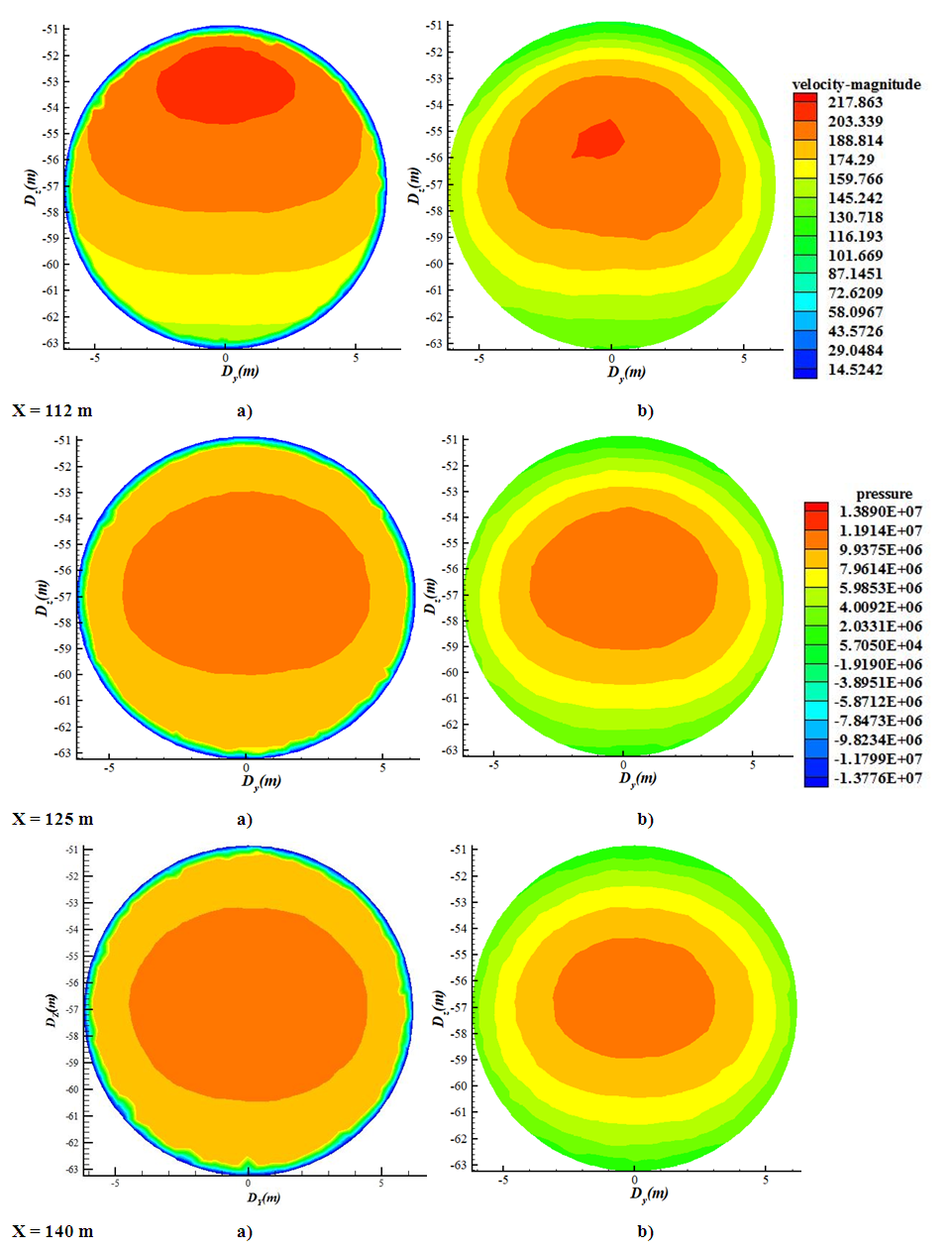 | Figure 7. Velocity (a) and pressure (b) field in section 3 |
3.3. Comparative Studies
Several studies are carried out on penstocks and these on various aspects. However, the structure of the flow remains one of the unknown parameters of the operation of the structure, because it is difficult to observe. As the interest of these studies relates to improving the performance of the entire structure, they are therefore essential on such a structure having been the subject of enormous expenditure and being classified as a risk structure. It is with this logic that Wang et al. [8] studied the velocity of the flow in the penstock entrance by the ultrasonic method in the Three Gorges dam. We compare our results with those obtained within the framework of this work as shown in the figure below.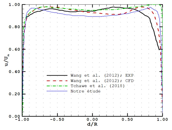 | Figure 8. Penstock velocity profile for Wang et al. [8], Tchawe et al. [9], and this study |
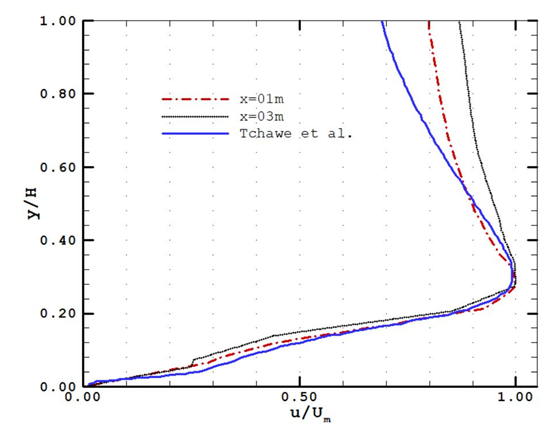 | Figure 9. Profile of velocities near the wall for the present study and that of Tchawe et al. [9] |
The arrangement of their probes may explain the error observed on the curves. However, from the results obtained within the framework of this work, including that presented in Figure 5 above, we validated our model. We then compared the flow structure upstream of the intake with that obtained in a previous work; this conforts us in the model used as we can see in the figure 6.The velocity profiles are consistent towards the lower wall, with a peak observed in the same interval. The difference observed towards the upper part of the profiles is justified by the modifications made to the configurations of the structure.In order to present the closeness at the level of the dynamic field, we compared our study with that of Adamkowski et al. (2009) [10], as shown in Figures 10a and 10b below. The goal in their studies was to measure flow using the pressure-time method in a three-section curved penstock like ours, but with a reduced diameter and longer length. It was equally question to evaluate the results obtained numerically on these structure.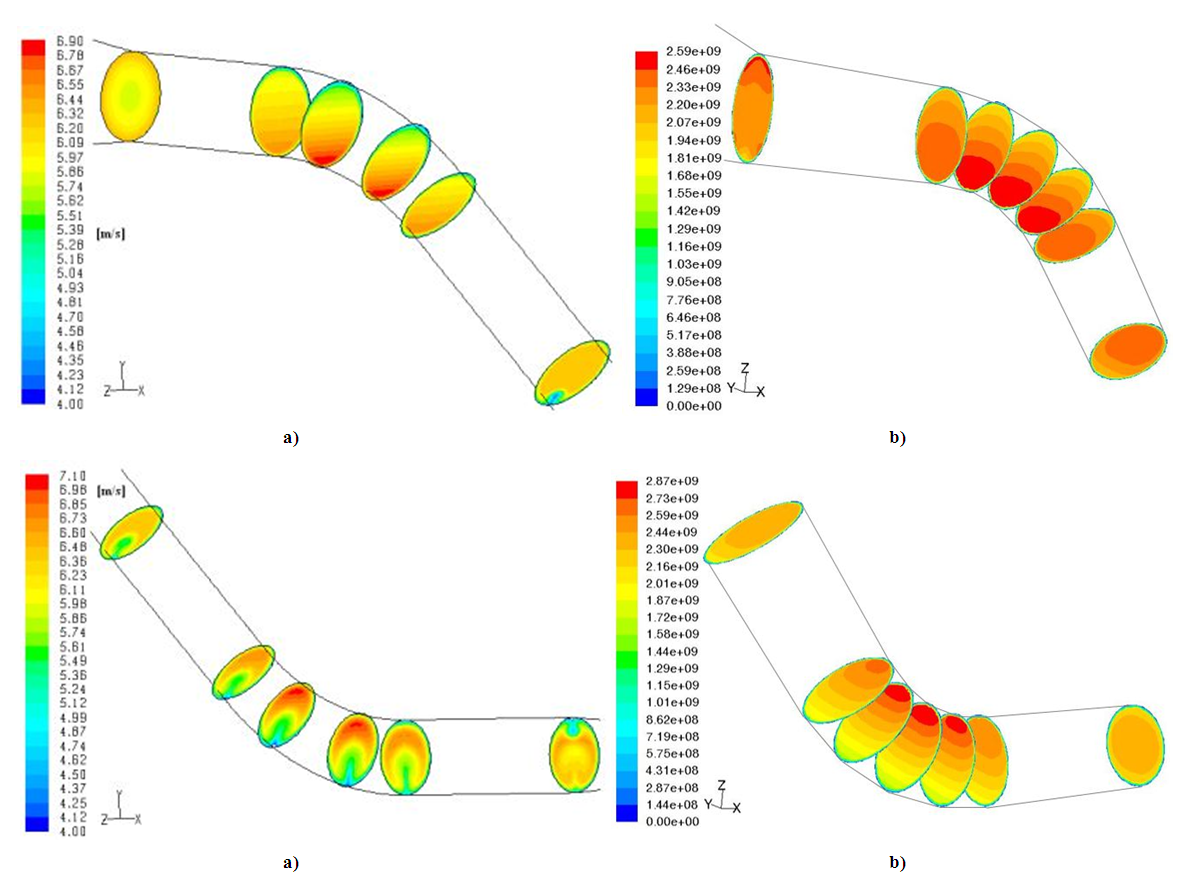 | Figure 10. Velocity field in driving for Adamkowski et al. [10] (a), and the present study (b) |
Thus, the general flow structure is found on both studies with the high velocity layers near the walls of the intake, folded towards the upper part in the second section and concentrated towards the innerside on each elbow. Likewise, these layers are located towards the axis of the pipe at the exit of the penstock in both researches. These observations are only possible thanks to the numerical approach which allows us to visualize the structure of the flow at each point in the pipe. According to ASME, having fully developed turbulent motion requires a straight line at least 10 times the diameter of the pipe; which is not the case in the two studies.
4. Conclusions
For us in this work, it was question to determining the dynamic field in the penstock of the Three Gorges dam in China, the objective being to determine the structure of the flow in this pipe using a numerical approach. We have therefore chosen the FLUENT calculation code, which is the most widely used in the world of hydraulic and particularly in hydroelectric dams. From the results obtained, we observe the constant velocity upstream of the dam until near the water intake at a distance of about 15m upstream. Its structure retains its asymmetric character in the different sections that constitute driving with maximum velocitys on the innerside of the different elbow. We also observed layers of non-zero pressure in the penstock, far from the walls; substantially coaxial and positive iso-pressures in high velocity zones, with a maximum directed towards the center of the penstock. A phenomenon that still goes against the high velocity-low pressure hypothesis. This new phenomenon can be justified by the geographical arrangement of the penstock, associated with its large diameter.
ACKNOWLEGDEMENTS
A special acknowledge to the University Institute of the Gulf of Guinea-Cameroon and its Founder Mr Louis Marie DJAMBOU (rest in peace) for his contribution in the development of this work.
References
| [1] | Tchawe T., (2019), "Etude et caractérisation du frottement turbulent dans la conduite forcée et dans le barrage de prise d’eau d’une station hydroélectrique: cas des barrages du Cameroun". Thèse en Génie Mécanique et Productique / Ingénierie des Equipements et Productique, Université de Ngaoundéré. |
| [2] | Singhal M. K. & Kumar A., (2015), "Optimum Design of Penstock for Hydro Projects". International Journal of Energy and Power Engineering, Vol. 4, No. 4, 2015, pp. 216-226. |
| [3] | Wilson D. Turbulence modeling for CFD. DCV industries, 2nd Edition, 1998. |
| [4] | Von Karman T., (1934), "The fundamentals of the statistical theory of turbulence". Journal of Aeronautical Science, 4, 131-138. |
| [5] | Tchawe T., Djiako T., Kenmeugne B., Tcheukam-Toko D., (2018), "Numerical Study of the Flow Upstream of a Water Intake Hydroelectric Dam in Stationary Regime ". American Journal of Energy Research, 2018, Vol. 6, No. 2, 35-41. |
| [6] | Boussinesq, (1877), "Théorie de l’écoulement tourbillonnant et tulmultueux des liquides". Paris, 1897. |
| [7] | Prandtl, (1932), "Ergebnisse Göttingen". 1932, 4, p. 18. |
| [8] | Wang C., Meng T., Hu H., Zhang L., (2012), "Accuracy of the ultrasonic flow meter used in the hydroturbine intake penstock of the Three Gorges Power Station". Flow Measurement and Instrumentation, 25: 32–39. |
| [9] | Tchawe T., Djiako T., Kenmeugne B., Tcheukam-Toko D., (2018), "Numerical study of flow in the water inlet of the penstock of a hydroelectric dam", International Journal of Current Research, Vol. 10, Issue, 07, pp.71061-71066, July, 2018. |
| [10] | Adamkowski A., Krzemianowski Z. & Janicki W., (2009), "Improved Discharge Measurement Using the Pressure-Time Method in a Hydropower Plant Curved Penstock". Journal of Engineering for Gas Turbines and Power, vol. 131, pp.6. |
| [11] | Fluent (2006). User manual 6.3.26. |

 Abstract
 Reference
 Full-Text PDF
 Full-text HTML