-
Paper Information
- Previous Paper
- Paper Submission
-
Journal Information
- About This Journal
- Editorial Board
- Current Issue
- Archive
- Author Guidelines
- Contact Us
International Journal of Energy Engineering
p-ISSN: 2163-1891 e-ISSN: 2163-1905
2020; 10(3): 80-89
doi:10.5923/j.ijee.20201003.02

A Comprehensive Forecasting, Risk Modelling and Optimization Framework for Electric Grid Hardening and Wildfire Prevention in the US
 Abstract
 Reference
 Full-Text PDF
 Full-text HTML
1School of Engineering, University of Kansas, Overland Park, USA
2Department of Biostatistics & Data Science, University of Kansas, Kansas City, USA
Correspondence to: Soham Ghosh, School of Engineering, University of Kansas, Overland Park, USA.
| Email: |  |
Copyright © 2020 The Author(s). Published by Scientific & Academic Publishing.
This work is licensed under the Creative Commons Attribution International License (CC BY).
http://creativecommons.org/licenses/by/4.0/

Historical wildfire patterns have experienced a recent shift in terms of its scale and intensity. Through the continuing advancements in electrical protection technology, statistical forecasting methodologies, availability of meteorological field data, and regional risk-modelling, wildfire management practices can be made more proactive in the United States and around the globe. To create a comprehensive and practical operating framework, an advanced seasonal autoregressive integrated moving average time series modelling technique for wildfire forecasting is explored. These regressive models, due to their mathematical accuracy has been used in many engineering and scientific applications. The study presented here was done using a qualitative investigation approach to wildfire data. Computer automated grid search techniques were developed to determine suitable seasonal regressive model hyper-parameters. With the usage of power transforms to fit skewed statistical models under study, it is found that a much more accurate and computationally efficient model can be generated. Statistical forecasts and regional risk mapping techniques can influence strategic operational practices for regional and local fire authorities. Concepts that can enhance power system protection and electrical grid hardening are explored and practical guidelines to help electrical utilities improve electrical grid operations are provided. Many benefits of using distributed energy resources are discussed and an optimal power flow involving these resources is formulated to help grid operators preserve system stability under these wildfire scenarios.
Keywords: Grid maintenance planning, SARIMA, Auto-regressive models, Forecasting, Wildland-urban interface, Risk-model, Distributed energy resources
Cite this paper: Soham Ghosh, Sreejata Dutta, A Comprehensive Forecasting, Risk Modelling and Optimization Framework for Electric Grid Hardening and Wildfire Prevention in the US, International Journal of Energy Engineering, Vol. 10 No. 3, 2020, pp. 80-89. doi: 10.5923/j.ijee.20201003.02.
Article Outline
1. Introduction
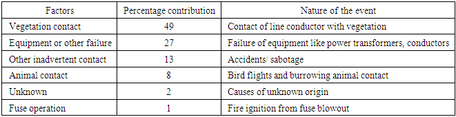
- Effective wildfire policies are of paramount importance for natural resource management and to ensure public health and safety. In the US, historical patterns of these fires were mostly caused due to lightning or burning by the native population. However, recently these historical patterns have shown significant changes in terms of the size, intensity, and duration of the wildfires [1,2]. The changes in the historical patterns are mostly attributed to a synergy of natural and human causes. Changes in rainfall patterns and snowpack, increased periods of drought, and replacement of native grasslands with invasive species are rapidly increasing the potential of future wildfires. To add to the problem, population growth is pushing residential development into forested and semi forested areas which are recurrent spots for wildfires [3–5]. One key issue of these wildland-urban developments is the growing need for electrification of these areas with transmission, distribution, and substation assets. The inherent risk of fires due to electrical faults and other maintenance issues of these assets makes the management of the wildfires in these urban fringe areas challenging and costly. For instance, from 2000-2016, the electrical asset-related damages for utilities in California is in upwards of $700 million [6] mostly reported along these wildlife-urban fringe areas. Understanding and statistical forecasting of these wildfire time-series trends can demonstrate a pathway for future energy policies and utility level decision making on electrical maintenance and planning.A risk event frequency study [7] from 2015-2017 over the high fire threat districts (HFTD) of California, US has revealed the key contributing element for over four hundred wildfire events as summarized in Table 1. As one can observe, contact of live conductors with vegetation, and equipment and hardware failures are reasons that are potentially controllable with human interference yet have contributed greatly to the cause of massive wildfires. From this observation greater focus has been given to the role of vegetation in increasing forest fire risk and preventive maintenance solutions have been likewise investigated.
|
2. Automated Grid Search and the Use of Power Transforms
2.1. Data Acquisition and Pre-processing
- The study employs a time series data spanning from 1992 to 2015, collected out of Forest Service Research Data Archive, United States Department of Agriculture [17]. The wildfire records of this data set were acquired from federal, state and local fire organizations. The available data-set has over one million forty-eight thousand entries with the granularity at a day level. From the given data-set, the dates at which a given wildfire was observed and the size of the burnt area are the primary area of interest for this study. Most commonly available data-sets suffer from random missing observations. The common approach to deal with random missing observations is to insert an estimated value. For this study, the weighted average of p observation points before and after the missing values has been used, as shown in Equation 1. Furthermore, for a discussion on observations with systematic missing patterns [18] provides an excellent reference.
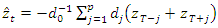 | (1) |
 and
and 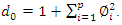 Following the data pre-processing steps, some descriptive statistical tools were used to visualize the data. Figure 1 shows a box and whisker plot of the monthly wildfire trend, with a clear indication of high median count for the summer and early fall season, and a near-zero median count during the winter season. This observation would be of some importance for the structuring the energy policy recommendations later in Section 4 of this study.
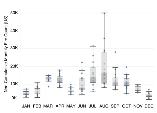 | Figure 1. Box and whisker plot summary of the US monthly wildfire count |
2.2. Automated Grid Search Approach to Determine SARIMA Model Hyperparameters
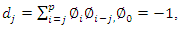
- The building blocks of an ARIMA (p,d,q) model are the autoregressive order p: AR (p) model and moving average order q: MA (q) model. An AR (p) model is a discrete time series linear equation, as described by Equation 2, where p is the model order and
 are the coefficients with
  as error term.
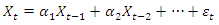 | (2) |
 , we can generalize AR (p) model from Equation 2 as shown in Equation 3.
 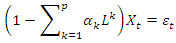 | (3) |
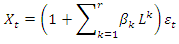 | (4) |
 as error term.
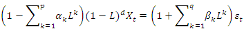 | (5) |
 | (6a) |
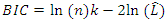 | (6b) |
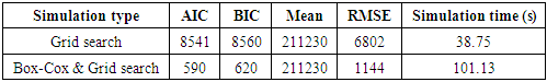
 is the maximum value of the likelihood function of the model, n is the number of data points and k is the number of free parameters to be estimated. The second term in Equations 6a and 6b penalizes the ARIMA model for too many parameters. As such, to improve computation efficiency the approach used here is to exit the nested grid search loop if the numerical value of the AIC or BIC converges to a high number after several iteration steps.A final step before a grid search simulation is executed to establish if the given data has a seasonal trend. From several decomposition techniques that are discussed in the literature [23,24] a seasonal and trend decomposition using loess (STL) technique was used to verify seasonality. The relative merit of this decomposition technique is that its robust to outliers, a property ideal to analyse wildfire data. With seasonality observed in the data-set three more hyperparameters, P, D, and Q are defined for the seasonal component of the model. Thus, the complete SARIMA (p,d,q)(P,D,Q,m) model under investigation have trend component parameters of p, d and, q for the autoregression, difference and moving average portions and P, D, Q and, m due to the seasonal component for autoregression, difference, moving average and seasonal period.With a grid search simulation on the wildfire data-set with 288 entries, with an aggregated granularity at a monthly level, the hyper-parameters for this SARIMA model are found to be (0,1,1)(1,0,1,12) along with a total computation time of 38.76 seconds on standard Intel i5 hardware. The model performance in terms of standard statistical metrics and numerical values of AIC, BIC are summarized in Table 2. Figure 3 shows the prediction performance for 24 months with seasonal high during the summer months.
2.3. SARIMA Model Parameter Selection Using Power Transforms
- Real-life data as obtained from [17] rarely tend to be normally distributed and is typically skewed. The issue with trying to fit a regression model on a skewed data is often complicated and not encouraged since the regression assumptions are violated. Decision tree-based classification techniques can be used to fit this kind of data, without requiring the data to be transformed, as noted in reference [25].For auto-regressive based models, power transforms like Box-Cox or Yeo-Johnson transformations [26,27] are typically used to normalize a skewed distribution. We can use these transforms to our advantage to normalize our data-set for better fitting our model. A two-parameter Box-Cox transformation as defined in Equation 7 is used to transform the wildfire study data. The transformed data is sequentially fitted into a SARIMA model using the same grid search technique described in Section 2.2. Once the transformation is applied and the grid-search algorithm is executed, it is imperative to re-transform the data back to get to the original scale.
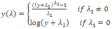 | (7) |
 are the transformation parameter. It should be noted that
  requires a special definition and is the log of the data itself. Statistical analysis on the original data-set from [17] reveals skewness in Figure 2a, as expected with phenomenon like wildfires. The given data-set is normalized with a Box-Cox transformed, as described by Equation 7 and is shown in Figure 2b. Readers should be aware that due to the nature of the Box-Cox transformation, only positive valued data-set or data-set with non-negative values can be transformed which is ideal for wildfire data-set. With a grid search simulation on the Box-Cox transformed wildfire data-set with 288 entries, aggregated to a monthly granularity level, the hyper-parameters for the Box-Cox transformed SARIMA model were found to be (2,0,0)(2,0,1,12) with a total computation time of 101.13 seconds on standard Intel i5 hardware. The model performance in terms of standard statistical metrics and numerical values of AIC, BIC are summarized in Table 2. Figure 3 shows the prediction performance for 24 months with a seasonal high during the summer months.
|
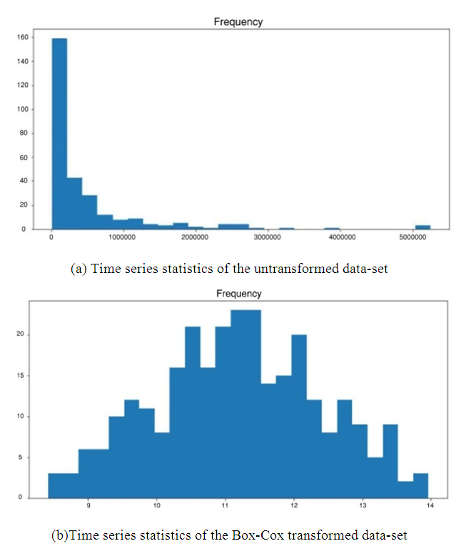 | Figure 2. Critical statistics of the time series data |
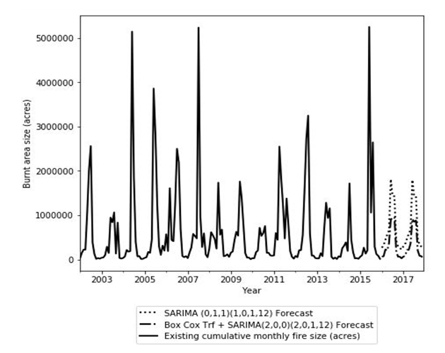 | Figure 3. Forecast performance of SARIMA and transformed SARIMA models |
3. Numerical Performance Evaluation
- Before evaluating model performance, some notes on forecasting very long and extremely granular times series are presented. It is a general observation that most time series model do not work well for a long and extremely granular data-set. Wildfire data obtained from [17] consists of multiple entry for each date-time index and recorded at a twenty-four-hour level of granularity. These individual entries should be aggregated to an acceptable level of granularity, to improve computation time and retain forecasting objective. For this study, the time stamp data were aggregated to the level of granularity at a monthly level, which aligns well with the objective of this study.For model evaluation, the entire data-set is broken into training and testing data and the model is trained on the initial eighty percentage of the data. The forecasting performance of both the SARIMA (0,1,1)(1,0,1,12) model and the Box-Cox transformed SARIMA (2,0,0)(2,0,1,12) model has been measured by root mean square error (RMSE) on the test set of the wild fire data-set. For a detailed discussion of these evaluation metrics, readers are encouraged to refer [28]. The improvement of the proposed Box-Cox transformed SARIMA (2,0,0)(2,0,1,12) model over the benchmark regular SARIMA (0,1,1)(1,0,1,12) model can be seen from Table 2. It is observed that without the transformation, a straightforward nested grid search algorithm yields a relatively high information criterion and higher root mean square error on the test data. Also, the overall performance of the two models is superior, given the low RMSE compared to the data mean. From these observations, it can be suggested that suitable transformation methods should be explored before fitting naturally skewed data-set for robust model fitting. An initial descriptive statistical analysis should also be conducted, as discussed above, on skewed data-sets to establish whether the data is left or right-skewed.
4. Recommendations on Future Energy Policies
4.1. Operating Framework for Local and Regional Fire Departments
- This section deals with developing a workable risk-model for the local and regional fire departments. The proposed risk-model for regional risk assessment is divided into three parts: the working voltage level of the electrical asset being analysed, the position of the active zone of the flame in regard to the electrical conductors, and the effect of temperature, relative humidity and ionization in form of air pollution.The idea of the first component of the risk-model is to establish transmission security for important 500, 345 and 138 kV lines since an outage on these lines have major impacts on grid stability and on public welfare. Since the voltage levels and power carrying capacity of electrical networks are typically non-linear, a logarithmic scale is used for this model. In Equation 8,
 is the sensitivity factor to be chosen by fire analyst and n represents a scaled integer corresponding to a voltage level.
 | (8) |
 is the sensitivity factor to be chosen by fire analyst and
  represent the height of the energized electrical asset from the terrain level.
 | (9) |
 typically tend to increase the temperature factor by providing forest fuel for a wildfire burn and is included as a risk-parameter. Further, higher relative humidity (RH) tends to reduce wildfire risk by a square inverse factor. Last, experimental studies in a controlled environment have shown a higher risk of electrical breakdown in the presence of atmospheric contaminants (τppm) [30] and is included in the risk-model. The combined model with all the above parameters included is shown in Equation 10. Like the sub-models discussed an operator adjustable sensitivity factor of
  is added into the equation.
 | (10) |
 and
and  The model used a scoring system and the heat-zones in Figure 4 represents a unique score for each county for all the forty-eight states. High risk areas are detected whenever the combination of high forest coverage
  low relative humidity (RH), high ambient temperature (Tambient) and high atmospheric contamination (τppm) are favourable from a multiplicative standpoint. As such, from Figure 4, US states like California, Nevada, Arizona and Oregon having the right mix of these factors are more susceptible to forest fires as compared to other US states like Virginia and Tennessee, where high relative humidity creates an unfavourable wildfire condition.
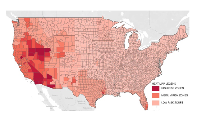 | Figure 4. Heat map showing modelled risk of wildfires in US for 138 kV transmission lines |
4.2. Operating Framework for Entities Managing Transmission and Distribution
4.2.1. Upgrade System Protection and Relaying Schemes
- The strategical operational practices: combining forecasting wildfires from time series analysis of historical data and accurate regional risk mapping can help shape local and regional fire management policies. However, grid operators can do much more than solely relying on these strategic practices for grid operation and can invest to upgrade system protection and harden the overall system, as would be discussed next.The issue of wildfires as seen in the introductory section of this article revealed that a major portion of these incidents is caused due to broken or downed conductors. Fault scenarios arising from these faults are typically single line to ground (SLG) in nature. These SLG faults are unbalanced and must be analysed using symmetrical component analysis technique. An excellent discussion of symmetrical component analysis can be found in [32], and the results from such an analysis is summarized in Equation 11a-c, where Vf is the pre-fault voltage, Zf is the fault impedance and
 are the zero, positive and negative sequence impedance.
 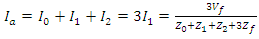 | (11a) |
 | (11b) |
 | (11c) |
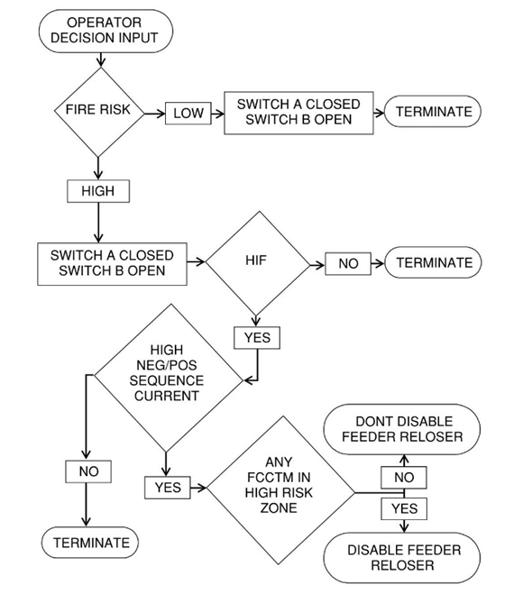 | Figure 5. Flowchart to guide disabling reclosure and fast acting fuse switching |
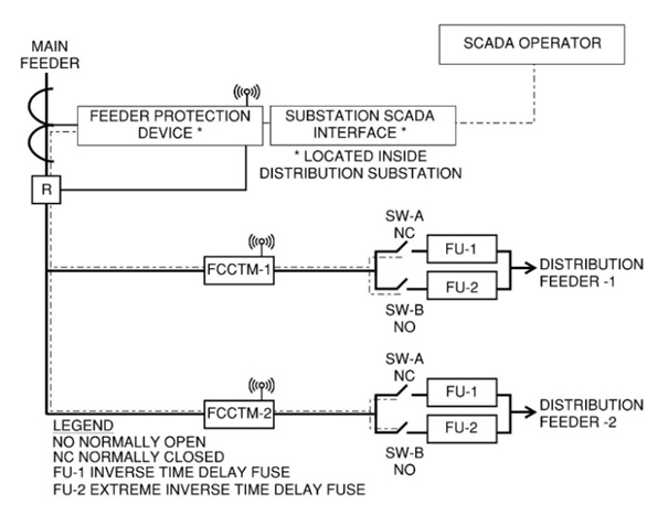 | Figure 6. Guided reclosing using field FCCTM signals |
4.2.2. Other Effective Techniques to Harden the Overall Electrical Grid
- A few non-conventional approaches are discussed in this section, which has the potential to harden the electrical network against wildfires.To enhance electrical grid resilience regular oil filled instrumentation transformers can be replaced with its optical counterpart, in high wildfire risk zones. These compact optical transformers have superior seismic performance due to its light weight and footprint and can be used to adapt to a wide range of electrical turns ratio. Other major advantages of these systems are its linear performance due to the absence of iron core saturation and galvanic isolation of high voltage lines. Unlike a capacitor coupled voltage transformer (CCVT) an optical transformer relies on the physical phenomenon of Pockels effect [35] and can be used to measure harmonic contents at interfacing substations and point of interconnections.Though instrumentation transformers can be replaced by optical transformers in limited scenarios, oil cooled power transformers possess its unique challenges in terms of wildfire risk. Engineered K-class ester based mineral oil [36] with extremely low flammability can be used to replace existing transformer oil during routing or emergency maintenance, to reduce fire propagation through utility transformer assets in high risk areas. These engineered ester-based oils can have fire points as high as 680°F and can be tuned to comply with industry testing standards as IEEE C57.154 [37] for high temperature insulation systems.
4.3. Operating Framework for Entities Managing Distribution Energy Storage Assets
- Distributed energy storage systems (DESS) can contribute in forming a bare backbone transmission and distribution network with decentralized energy pools. Since the reliability of the transmission and distribution network is ensured around peak wildfire period of summer and early fall, due to the maintenance and upgrades done in the previous season as outlined in Section 4.1, developers can use this timeframe to line up DESS projects.During these wildfire events, reasons to promote the use of DESS in enhancing grid flexibility are many. During a wildfire incident a DESS resource can support to maintain security constrained power flow, help prevent anti-islanding by real power support, and help system operators to reconfigure the network remotely and still maintain overall grid stability. After the course of a wildfire, a DESS cluster of distributed generation (DG)/ demand responsive load (DR) can be used to black start tripped generators and for other load restoration. As such these DESS clusters can help in a much faster recovery of the affected electrical grid. Readers should be aware however of the potential risks involved with energy storage technologies from a fire safety standpoint and should have these resources installed at site in accordance to NFPA 855: standard for the installation of stationary energy storage system [38].Furthermore, during daily grid operations, often time in practice a combination of reduced transmission line loading along with support from distributed generation and demand-responsive loads can help the grid ride-through an emergency condition. The rest of this section presents a discussion of a DC optimal power flow formulation under a combination of these stressed situations, to ensure the most economical allocation and dispatch of generations and loads. The formation discussed henceforth considers the presence of both demand-responsive loads and distributed generation in micro-grid nodes which are connected to the main electric grid. There are many DC optimal power flow formulation available in the literature. For instance [39] presents a DC optimal power flow formulation (DCOPF) to analyse N-1 contingency analysis with optimal transmission switching. Each DC optimal power flow formulation has its own set of objective function and boundary conditions, and hence the corresponding primal-dual interpretation of every problem is unique to the situation.The optimization problem assumes that all generation costs are linear and a lower bound of zero active power production from these generating resources. The optimization problem is developed as follows:
 | (12a) |
 | (12b) |
 | (12c) |
 | (12d) |
 | (12e) |
 | (12f) |
 | (12g) |
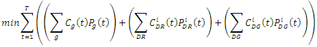
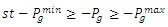
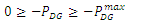
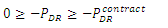
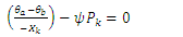
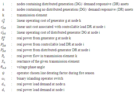 The objective function and constraints of the of the above optimal dispatch formulation are explained below:Equation 12a: Objective function - The objective function of this formulation is to minimize generation cost and hence find the most economical generation level, that can provide a feasible solution during grid disturbance as these. The first term of the minimization objective function represents the cost of generation from convention generating units. The second term of the objective function represents the cost of purchasing demand response reserve from a demand response load. Typically, these can be done through contractual agreements and can be renewed as required. The last term represents the cost of generation from the distributed resources which can look very different from its utility generation counterpart.Equation 12b: Utility generation constraint - This constraint captures the practical loading of utility generators. By its very nature these generators are often bound in their minimum and maximum real power output levels set-forth by manufacturer warranty agreements.Equation 12c: Distributed generation constraint - The given constraint captures the maximum power limit of the distributed generators. Note that since these are usually modular power electronic controlled devices, the lower operating limit is not of concern and is chosen to be zero.Equation 12d: Demand response contractual constraint - The demand response contractual constraint captures the contractual agreement made between the system operators and the owners of the demand responsive load. This constraint can be changed based on season agreements.Equation 12e: Transmission element thermal rating constraint - The power flow constraint is a linear approximation of the actual line flow constraint and consists of the reactance
  of the transmission element and the voltage phase angle between its two ends
  . The term
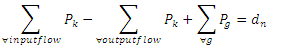
  is an active derating factor that can be chosen by the grid operator to de-rate certain transmission elements in the path of high fire risk zones.Equation 12f: Node power balance constraint - The node power balance constraint involves boundary condition between power inflow and outflow in a transmission element, generation and load levels at a node.Equation 12g: Island operation constraint - A feasible operational islanded microgrid needs to balance its load in case the operator must island an electric region to preserve grid stability. The active load demand of this microgrid should be less than or equal to the available real power from its distributed generation and demand responsive load resources. The term
  is a binary state indicator and equals zero in an active island condition.As can be seen from this formulation, the system operator can ensure better ride-through of the electrical grid under system disturbance with a combination of strategies as reduced line loading, contractual demand responsive load agreements and islanded microgrid operations in a small scale in probable high fire risk zones. On the other hand, DESS developers can actively engage to increase the preparedness of the electric network to disturbance as these through simulation studies and strategic placement of DESS resources.
5. Conclusions
- A combination of statistical forecasting, risk-modelling, and power flow optimization framework has great potential to improve the impacts of wildfires on public welfare and safety. A proactive multi-faceted approach at different levels and implementation of design codes and standards can make the bulk power system resilient to these phenomena. This paper explores the practical challenges of numerical forecasting of wildfire data and provides solutions to reproducible accurate forecasting. Fire operators can use the framework discussed in this paper at a level of granularity of their geographical region for future planning and related investment decisions. Electrical utilities can implement a multi-year approach to systematically upgrade its protection schemes with advanced protection and relaying schemes presented in this paper. Along with these policy recommendations, a feasible optimization framework of combined distributed generation, demand-responsive loads and adjusted line capacities can help system operators ride-through these challenging situations.