Isaiah Kimutai1, Paul Maina2, 3, Augustine Makokha1, 3
1Department of Energy Engineering, Moi University, Eldoret, Kenya
2Department of Mechanical & Production Engineering, Moi University, Eldoret, Kenya
3Africa Center of Excellence in Phytochemicals, Textile and Renewable Energy, Moi University, Kenya
Correspondence to: Isaiah Kimutai, Department of Energy Engineering, Moi University, Eldoret, Kenya.
| Email: |  |
Copyright © 2019 The Author(s). Published by Scientific & Academic Publishing.
This work is licensed under the Creative Commons Attribution International License (CC BY).
http://creativecommons.org/licenses/by/4.0/

Abstract
The increasing cost of energy has caused the energy intensive industries to examine means of reducing energy consumption in processing in order to remain competitive both in local and global markets. This paper presents a method for modeling and optimizing energy use in textile manufacturing using linear programming (LP). A linear programming model has been developed which meets the finished product requirements at a minimum cost of energy used in the process subject to different operational constraints. To develop the model, data required were collected through energy audit of the plant. It is through energy audit that constraints and products manufactured were identified and used in the development of the model. Constraints come in the form of system material balance equations and output production demands. Material balance equations and energy balance are the main features of the model. The model will determine optimum values for the process design variables, so as to achieve minimum cost. Sensitivity analysis of the model determines how the optimal production values (optimal solution) are affected by changes in prices of the resources (objective function coefficients).
Keywords:
Optimization model, Linear programming, Process industry, Energy audit, Material balance, Energy balance, Sensitivity analysis, Kenya
Cite this paper: Isaiah Kimutai, Paul Maina, Augustine Makokha, Energy Optimization Model Using Linear Programming for Process Industry: A Case Study of Textile Manufacturing Plant in Kenya, International Journal of Energy Engineering, Vol. 9 No. 2, 2019, pp. 45-52. doi: 10.5923/j.ijee.20190902.03.
1. Introduction
Increasing energy demand, high energy costs and scarce availability of resources demands energy conservation and optimal utilization of energy inputs across all energy consuming sectors in order to reduce energy consumption and related energy costs. It is through adoption of energy management that industries can address energy matters in order to remain profitable and competitive both locally and globally especially for energy intensive industries such as textile manufacturing. A good and sound energy management ensures optimum utilization of energy inputs in a plant such as electricity and fuel.Energy management applies to resources as well as to the supply, conversion and utilization of energy. Essentially it involves monitoring, measuring, recording, analyzing, critically examining, controlling and redirecting energy and material flows through systems so that least power is expended to achieve worthwhile aims [1]. Therefore, energy management modeling may be defined as an investigation of the allocation of energy resources over time by determining the cheapest and most efficient way of meeting final demands with available and potential resources and technologies.Energy systems are usually complex systems within which elements and subsystems are highly correlated, and their behavior is hardly predictable without application of exact mathematical methods. Under the conditions of limited energy sources, the optimal economic effects of an energy process can be achieved only if optimal relationships of all components of the system are kept permanent. In addition, under the conditions of increased prices of energy systems, optimal operation of energy systems tend to be very relevant [2].Textile manufacturing is complex because of the wide variety of substrates, processes, machinery and apparatus used, and finishing steps undertaken. Different types of yarns, methods of fabric production, and finishing processes (preparation, printing, dyeing, chemical/mechanical finishing, and coating), all correlate in producing a finished fabric. Textile manufacturing is an energy intensive process. Especially in times of high energy price volatility, improving energy-efficiency should be a primary concern for textile plants [3]. Fig. 1 shows product flow diagram depicting the various textile processes that are involved in converting raw materials in to a finished product.Modelling of complex problems can lead to better decisions by providing decision makers with more information about the possible consequences of their choices. Hence, the use of energy models as tools for dealing with complicated problems can help decision makers to overcome this difficulty. Energy models are useful mathematical tools based on the system approach and the best model should be determined based on the problem that decision makers endeavour to solve [4].Optimization models try to define the optimal set of technology choices to achieve a specific target at minimized costs under certain constraints leaving prices and quantity demanded fixed in its equilibrium. Every modelling approach abstracts to a certain degree from reality using stylized facts, statistical average figures, past trends as well as other assumptions. Consequently, energy models represent a more or less simplified picture of the real energy system and at best they provide a good approximation of today’s reality [5]. An optimization model defines the required input data, the desired output, and the mathematical relationships in a precise manner.There are many types of optimization models such as linear programming, nonlinear programming, multi-objective programming, and bi-level programming. Linear programming has a tremendous number of application fields. It has been used extensively in business and engineering, in the areas of transportation, energy, telecommunications, and manufacturing. It has been proved to be useful in modeling diverse types of problems in planning, routing, scheduling, assignment, and design. Linear programming is also heavily used in various management activities, either to maximize the profit or minimize the cost. It is also the key technique of other optimization problems. This model is defined by an objective function and one or more constraints which have linear formats [6].This paper develops a textile manufacturing plant industrial model which is designed to analyze and minimize energy costs for a system involving the manufacture of yarn, grey fabric and finished fabric with equipments using electricity, wood fuel and fuel oil. The most common problem in these industries involves allocation of limited resources among competing activities in the best possible (optimal) way. The objective is to develop mathematical models that meet the finished product requirements at a minimum cost of energy used in the process subject to different operational constraints.
2. Linear Programming
In recent decades, several models have been proposed in the field of energy management systems. These models have been used widely for optimal allocation of energy resources, technologies and services in accordance with the executive goals. Linear programming is one of several mathematical techniques that attempt to solve problems by minimizing or maximizing a function of several independent variables. The objective function may be profit, cost, production capacity or any other measure of effectiveness, which is to be obtained in the best possible or optimal manner. It concerns the optimum allocation of scarce or limited resources among competing activities, under a set of constraints imposed by the nature of the problem being studied [7]. These constraints could reflect financial, technological, marketing, organizational, or many other considerations.It was in 1947 that George Dantzig and his associates found out a technique for solving military planning problems while they were working on a project for U.S. Air Force. This technique consisted of representing the various activities of an organization as a Linear Programming model and arriving at the optimal programme by minimizing a linear objective function. Afterwards, Dantzig suggested this approach for solving business and industrial problems. He also developed the most powerful mathematical tool known as ‘Simplex Method’ to solve Linear Programming problems [8,9].Programming problems deal with the efficient use or allocation of limited resources to optimize certain desired objectives. Often, for each problem there exist a large number of solutions that satisfy the basic conditions. The best solution to a problem is selected based upon some overall objective that is included in the statement of the problem. The optimum solution is the one that satisfies the constraints of the problem and maximizes/minimizes the given objective [10].
2.1. Mathematical Formulation of Linear Programming Problem
There are four basic components of an LPP:1. Decision variables -The quantities that need to be determined in order to solve the LPP are called decision variables.2. Objective function -The linear function of the decision variables, which is to be maximized or minimized, is called the objective function.3. Constraints -A constraint is something that plays the part of a physical, social or financial restriction such as labor, machine, raw material, space, money, etc. These limits are the degrees to which an objective can be achieved.A linear programming problem (LPP) is an optimization problem in which(i) The linear objective function is to be maximized (or minimized);(ii) The values of the decision variables must satisfy a set of constraints where each constraint must be a linear equation or linear inequality;(iii) A sign restriction must be associated with each decision variable.Two of the most basic concepts associated with LP are feasible region and optimal solution.Feasible region –The feasible region for an LPP is the set of all points that satisfy all the constraints and sign restrictions.Optimal solution -For a maximization problem, an optimal solution is a point in the feasible region with the largest value of the objective function. Similarly, for a minimization problem, an optimal solution is a point in the feasible region with the smallest value of the objective function.
2.2. General Linear Programming Problem
A general linear programming problem can be mathematically represented as follows [10]:Maximize (or Minimize) Z = C1X1 +C2X2+…+CnXn Subject to,a11x1 + a1jxj+…+ a1nxn (≤, =, ≥) b1a21x1 + a2jxj+…+ a2nxn (≤, =, ≥) b2……………………………………ai1x1 + aijxj+…+ ainxn (≤, =, ≥) bi……………………………………am1x1 + amjxj+…+ amnxn (≤, =, ≥) bmand x1, x2,…,xn ≥ 0The problem is to find the values of xj’s that optimize (maximize or minimize) the objective function. The values of xj’s must satisfy the constraints and non-negativity restrictions. Here, the coefficients cj’s are referred to as cost coefficients and aij’s as technological coefficients; aij represents the amount of the ith resource consumed per unit variable xj and bi, the total availability of the ith resource.An LP problem can also be written in a compact form as follows [11]:Maximize (or minimize) the objective functionZ = CXSubject to m constraintsAX ≤ b, X ≥ 0The values in the X vector are called decision variables (the unknowns), and the values in the b vector are often called right-hand sides (RHS). The technique finds broad use in operations research.Linear Program Solver (LiPS v1.11.1 software.) was used to solve the energy problem. Linear Program Solver (LiPS) is an optimization package oriented on solving linear, integer and goal programming problems. It takes the optimization equation, variables and constraints as the input and generates the optimum solution as the output. It solves both minimization and maximization problems.The main features of LiPS are: Ø LiPS is based on the efficient implement-ation of the modified simplex method that solves large scale problems.Ø LiPS provide not just an answer, but a detailed solution process as a sequence of simplex tables, so you can use it for studying/teaching linear programming.Ø LiPS gives sensitivity analysis procedure-s, which allow us to study the behaviour of the model when you change its parameters, including: analysis of changes in the right sides of constraints, analysis of changes in the coefficients of the objective function, analysis of changes in the column/row of the technology matrix. Such information may be extremely useful for the practical application of LP Models.Ø LiPS provide methods of goal programming, including lexicographic and weighted GP methods, which are oriented on multi-objective optimization.
3. Production Process
Textile manufacturing consists of five main stages namely spinning, sizing/preparation, rewinding, weaving and wet processing (finishing). Each stage is made up of a group of machines used for different purposes. Textile process starts with yarn making in spinning and woven fabric (grey fabric) in weaving through to finished fabric in wet processing. The energy inputs used in textile processing are electricity as a common power source for machinery, wood fuel and oil fuel as a fuel for boilers which generate steam and heat. The first, third and fourth stages consumes only electricity to operate the mechanical devices while the second and fifth stage consume not only electricity but also fuel (wood and oil) to generate steam and heat energy. Figure 1 shows the five main stages involved in textile manufacturing, energy inputs and products processed in each stage.Analysis of each of the five processes with respect to energy, products and technologies are described below.Stage 1-Spinning ProcessSpinning is the first stage of textile manufacturing where raw materials (cotton, viscose and polyester) are processed into yarn. Raw materials are the main inputs of stage 1. The main processed product of stage 1 is yarn which is represented by X1 in figure 1 below. Depending on customer orders or forecast demands provided by marketing department part of yarn manufactured in stage 1 are sent to store as finished product represented by P1 and the rest sent to stage 2 for further processing. Spinning process is made up of several machines which include bale breaker, step cleaner, draw frame, carding and open end machine. Spinning process electricity consumption represents 48% of the total consumption in the plant and is the highest consumer of electricity among the five textile manufacturing processes. Average monthly electricity consumption in stage 1 is 43,942 kW.Stage 2-Sizing/PreparationThe input material of stage 2 is sent from stage 1 plus recycled material from stage 3. The product processed in stage 2 is illustrated as X2 in figure 1. 3% of the products processed in stage 2 are sent to stage 3 as wastes for recycling while 97% is sent to stage 4 for further processing. Sizing is the process of applying the size material on yarn. Size is a gelatinous film forming substance in solution or dispersion form, applied normally to warp yarns. Starch, gelatin, oil, wax, and manufactured polymers such as polyvinyl alcohol, polystyrene, polyacrylic acid, and polyacetates are applied to warp yarn to bind the fiber together and stiffen the yarn to provide abrasion resistance during weaving [12]. Other objectives of sizing include;1. To improve the breaking strength of the yarn2. To increase smoothness of yarn3. To protect the yarn from abrasion 4. To increase yarn elasticity5. To decrease the generation of static electricity6. To decrease hairinessThe process involves the use of wood fuel in fire-tube boiler to generate steam used for sizing yarn, that is treatment using starch solution and the use of electricity to operate warping machines. The wood fire-tube boiler efficiency is 17.35% with steam generation rate of 3TPH. Average monthly electric consumption in stage 2 is 5,400 kW.Stage 3-RewindingStage 3 is a recycling unit. Waste materials from stage 2 and stage 4 are processed to be used in stage 2 and are represented by X3. Waste materials are the remains of yarn during the transfer of yarn from cones to warpers beam and transfer of yarn from weavers beam on weaving. This stage consumes only electricity and the average monthly consumption is 4,147 kW.Stage 4-Weaving ProcessWeaving is the fourth stage of textile manufacturing where treated yarn produced in stage 2 is woven through weaving machines to produce grey fabric represented by X4 in figure 1. Depending on customer orders part of products processed at this stage are sent to store as finished product represented by P2 and the rest sent to stage 5. The main weaving machines used include Projectile, Rapier, Air-Jet and Water-Jet depending on the grey fabric required. The energy input of stage 4 is electricity and the average monthly electricity consumption is 14,428 kW.Stage 5 Finishing Process (wet processing)This stage is the last stage of textile manufacturing. The main processes in this stage include singeing, washing, de-sizing, scouring, bleaching, mercerizing, stentering, curing and dying (printing). The grey fabric from stage 4 is passed through various processes to achieve the ultimate product which is finished fabric represented by X5 in figure 1. 96% of products processed at this stage are sent to store as finished products represented by P3 and approximately 4% is wasted and not recycled. This last stage is also energy intensive since grey fabric passes multiple stages to meet customer demands. Thermal energy is of high demand in this stage especially in washing, dyeing, treatment and drying of the fabric and is supplied by thermo boiler and fire tube boiler by burning heavy fuel oil and wood fuel. Electricity is required to operate the machines such as thermostenter, jigger and scouring machine. The efficiency of thermo boiler used is 86.1% with an output of 1860 kW. Average monthly electricity consumption at this stage is 20,608 kW. 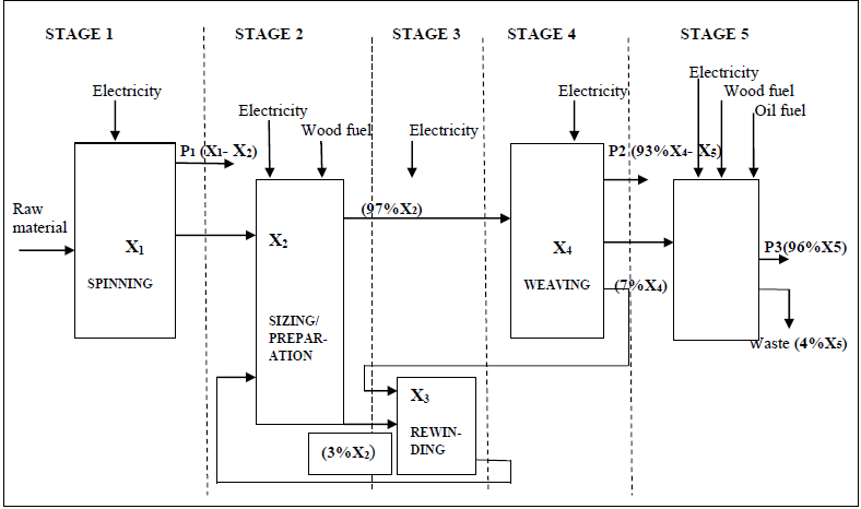 | Figure 1. Textile production flow chart |
4. Mathematical Model
Textile manufacturing is an energy intensive process and the objective of this study is to develop mathematical model that meet the finished product requirements at a minimum cost of energy used in the process subject to different operational constraints. The result of this process will yield a unique set of values that represent the quantities of products to be processed to meet monthly demands. Multi-stage linear programming is used in the development of the model. Material balance equations are the main features of multi-stage linear programming. Material balance equations are general expressions of material flows in the process.The linear programming problem is solved using the computer software called LiPS solver. To complete the analysis LiPS solver is used to perform a sensitivity study which shows the effect of changes in the different system parameters on the current optimal solution. This study then determines the range of a given element for which the solution remains optimal and, therefore, how sensitive the optimum solution obtained is to the parameter setting.Objective FunctionThe objective function is to minimize the total energy costs. | (1) |
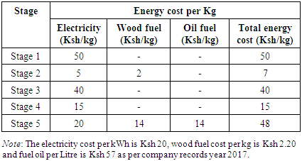
Where,C1 = Energy cost per unit of product to be produced in spinningC2 = Energy cost per unit of product to be produced in sizing/preparationC3 = Energy cost per unit of product to be produced in rewindingC4 = Energy cost per unit of product to be produced in weavingC5 = Energy cost per unit of product to be produced in finishingX1 = number of units of product processed at stage 1 in a monthX2 = number of units of product processed at stage 2 in a monthX3 = number of units of product processed at stage 3 in a monthX4 = number of units of product processed at stage 4 in a monthX5 = number of units of product processed at stage 5 in a monthThe objective function coefficients are the energy cost (electricity cost, wood fuel cost and oil fuel cost) per unit of product to be produced. These cost coefficients are calculated by multiplying amount of energy used to produce one unit of product by the cost of one unit of energy. Calculated coefficients of energy for the five stages of textile production are presented in table 1.Table 1. Energy cost coefficients for the model
 |
| |
|
Material Balance Equations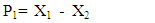 | (2) |
 | (3) |
 | (4) |
 | (5) |
 | (6) |
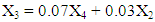
These constraints are the mathematical forms of the material flows of the process. Constraint (2) represents the material flow from stage 1 to finished product P1 and stage 2. The constraint (3) represents the waste material flow from stage 2 and stage 4 to stage 3 to be recycled. Constraint (4) represents the material flow from stage 2 to stage 4. Constraint (5) represents the material flow from stage 4 to finished product P2 and stage 5. Constraint (6) represents the material flow from stage 5 to finished product P3.Demand constraints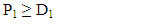 | (7) |
 | (8) |
 | (9) |
 | (10) |
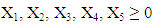
Where;P1 = number of units of finished product produced in stage 1 in a monthD1 = number of units of demand for product produced in stage 1 in a monthP2 = number of units of finished product produced in stage 4 in a monthD2 = number of units of demand for product produced in stage 4 in a monthP3 = number of units of finished product produced in stage 5 in a monthD3 = number of units of demand for product produced in stage 5 in a monthP1= X1 - X2P2= 0.93 X4 - X5P3= 0.96 X5Constraint (7, 8, and 9) ensures that the amount of finished product (P1, P2 and P3) cannot be negative. Constraint (10) represents that the amount of products processed in all the stages (X1, X2, X3, X4, and X5) cannot be negative.Time constraints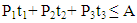 | (11) |
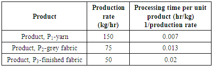
Where,t1= required processing time to produce unit of product P1t2 = required processing time to produce unit of product P2t3 = required processing time to produce unit of product P3A = available processing time in a monthConstraint (11) ensures that total production time in a month cannot exceed the available processing time in a month. Table 2 shows production rate of each product and the required processing time to produce one unit of product.Table 2. Production rate (kg/hr) and processing time per unit product (hr/kg)
 |
| |
|
4.1. Mathematical Model Data
The necessary for the model data include; Monthly energy consumption (electricity, wood fuel and oil fuel) for each stage, Monthly production for each stage, Forecast for future monthly demands, Capacity of the process and Material availability.The data required were obtained during energy audit from historical records, production process and production manager data. The necessary input data for the model are mainly the energy (electricity, wood fuel and oil fuel) used per unit of each product at each stage. The units of energy used are kWh, Litre and Kg for electricity, oil fuel and wood fuel respectively.
5. Results and Discussion
Linear Program Solver (LiPS v1.11.1 software) was used to solve the energy problem. This program solved the linear program problem and gave the ranges over which the cost coefficients and the right-hand side variables can vary without changing the optimality or feasibility of the problem.
5.1. Input Data
Minimize total cost (Z) = C1X1 +C2X2+C3X3 + C4X4+C5X5The terms of the linear programming objective function consist of the product of a cost coefficient and a variable. The cost coefficients have the units of Ksh/kg while the variable units are Kg. Therefore, each term and the total objective function have the units, Ksh. This means that the model minimizes the energy cost spent during production period.Minimize Z = 50X1 +7X2+40X3 + 15X4+48X5Subject to;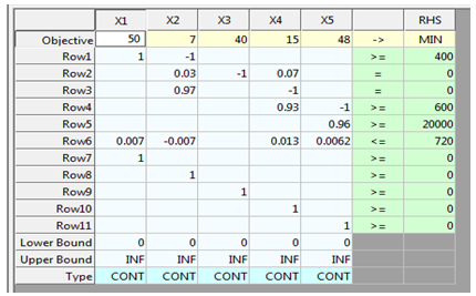 D1 = Product, P1 monthly demandD2 = Product, P2 monthly demandD3= Product, P3 monthly demandA = Available processing time in a monthThe monthly production demands in kg for the three products and available processing time in a month are given below;P1 = 400 kgP2 = 600 kgP3 = 20,000 kgA = 720 hrs
5.2. Output of the Model
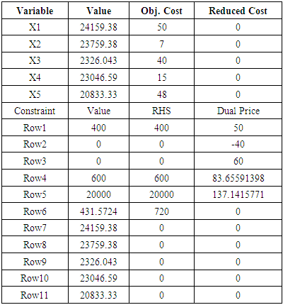
>> Optimal solution FOUND>> INFO: feasible solution FOUND after 5 iterations>> INFO: LiPS finished after 5 iterations and 0.03 seconds>> Minimum energy cost (Z) = Ksh 2,813,030 per monthTable 3. *** Results – Variables/Constraints ***
 |
| |
|
The model consists of 5 variables and 11 constraints. From table 3 above, we see that, the optimal solution is X1 = 24,159.4, X2 = 23,759.4, X3 = 2,326.04, X4 = 23,046.6 and X5 = 20,833.3 with optimal value of Ksh 2,813,030 per month. The minimum cost of product mix, when the electricity cost is Ksh 20/kWh, wood fuel cost Ksh 2.20/kg and fuel oil is Ksh 57/Litre, is Ksh 2,813,030 for the planned month. Results of the model provide optimum production mix with minimum energy cost.
5.3. Sensitivity Analysis
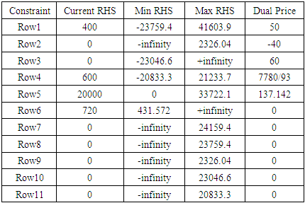
Sensitivity Analysis deals with finding out the amount by which we can change the input data for the output of our linear programming model to remain comparatively unchanged. This helps us in determining the sensitivity of the data we supply for the problem.This includes analyzing changes in:1. An Objective Function Coefficient (OFC)2. A Right Hand Side (RHS) value of a constraintThe sensitivity analysis for the monthly demand variables is shown in table 4 while sensitivity analysis for cost coefficients is shown in table 5 below.Table 4. *** RHS Range ***
 |
| |
|
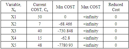
Table 5. *** COST Range ***
 |
| |
|
Table 4 lists the range of values for which the RHS (monthly production demand variables) may change without changing the optimality of the solution. Dual price is the amount in Kenya shillings per month by which the objective function value is increased per unit increase of the corresponding right hand side value (Kg/Month). In this research, if monthly demand of product P1 increases to 401 kg the objective function value would increase by Ksh 50 (the dual price) to Ksh 2,813,080 per month. Also, if monthly demand of product P2 increases to 601 kg the objective function value would increase by Ksh 84 (the dual price) to Ksh 2,813,114 per month. Similarly, if monthly demand of product P3 increases to 20,001 kg the objective function value would increase by Ksh 137 (the dual price) to Ksh 2,813,167 per month. Additional hour of production time will not affect the objective function value since the dual price corresponding to production time is zero. Table 5 lists the range of values for which the costs of the various energy sources may vary without changing the optimality of the solution though the objective function value may vary. Reduced cost indicates how much each cost coefficient would have to be reduced before the activity represented by the corresponding variable would be cost-effective. In this research, the reduced cost is zero for all cost coefficients, which shows no reduction is necessary.
6. Conclusions
The objective of this study was to apply the linear programming techniques to optimize energy use in textile manufacturing industry in order to minimize energy cost. For solving this problem, a linear programming model using simplex algorithm has been developed. The Linear programming technique determined optimum values for the process design variables, so as to achieve minimum cost. From the results the following findings were drawn:1) Spinning and wet processing constitute the bulk of energy cost in textile manufacturing. Results show that spinning process and wet processing represents 43% and 35% respectively of the total energy cost (optimal value).2) Sensitivity analysis shows that an increase in demand of yarn, woven fabric and finished fabric by 1 kg causes an increase of Ksh 50, 84 and 137 respectively on total energy cost.3) It has been shown that with the application of linear programming model, energy cost can be reduced considerably in textile manufacturing.Based on the findings of the research, the following conclusions were drawn:1) Optimal energy use in textile manufacturing can be achieved with the application of linear programming model. The system of equations can be expanded or reduced to accommodate any variety of system combinations.2) Energy saving and conservation measures in spinning process and wet processing is vital in order to minimize energy cost in textile manufacturing.3) The research is significant in the sense that it will assist the company in making corrective decisions well in time using the methods of linear programming. This will determine the future production patterns and outlook resulting in the establishment of new production units, while planning for energy cost minimization of the company.4) Although this research deals with minimizing energy cost in textile manufacturing industry, it can be applied to other process industries with similar processes.
References
| [1] | O'Callaghan, P. W., & Probert, S. D. (1977). Energy management. Applied Energy, 3(2), 127-138. |
| [2] | Dragićević, S., & Bojić, M. (2009). Application of linear programming in energy management. Serbian Journal of Management, 4(2), 227-238. |
| [3] | Hasanbeigi, A. (2010). Energy-efficiency improvement opportunities for the textile industry. |
| [4] | Neshat, N., Amin-Naseri, M. R., & Danesh, F. (2014). Energy models: Methods and characteristics. Journal of Energy in Southern Africa, 25(4), 101-111. |
| [5] | Herbst, A., Toro, F., Reitze, F., & Jochem, E. (2012). Introduction to energy systems modelling. Swiss journal of economics and statistics, 148(2), 111-135. |
| [6] | Zhang, G., Lu, J., & Gao, Y. (2015). Optimization Models. In Multi-Level Decision Making (pp. 25-46). Springer, Berlin, Heidelberg. |
| [7] | Akpan, N. P., & Iwok, I. A. (2016). Application of Linear Programming for Optimal Use of Raw Materials in Bakery. International journal of mathematics and statistics invention. Vol, 4. |
| [8] | Dantzig, G. B., & Thapa, M. N. (2006). Linear programming 1: introduction. Springer Science & Business Media. |
| [9] | Lewis, C. (2008). Linear Programming: Theory and Applications. Whitman College Mathematics Department. |
| [10] | Gass, S. I. (2004). Linear programming. Encyclopedia of Statistical Sciences, 6. |
| [11] | Lewis, C. (2008). Linear Programming: Theory and Applications. Whitman College Mathematics Department. |
| [12] | Medeiros, R. W., Corrigan, E. J., Tam, T. Y. T., Salem, E. H., Chen, J. Y., Reynolds, M. J., & Yasnowsky, J. K. (2004). U.S. Patent No. 6,796,337. Washington, DC: U.S. Patent and Trademark Office. |

 Abstract
 Reference
 Full-Text PDF
 Full-text HTML