M. K. Shirazi1, M. Joorabian2, A. Sadeghi3
1Faculty of Engineering, Islamic Azad University, Firoozabad Branch, Meimand center, Fars, Iran
2Faculty of Engineering S.C.U Shahid Chamran University Ahwaz, Iran
3Faculty of Engineering, Islamic Azad University, Kazeroon, Iran
Correspondence to: M. K. Shirazi, Faculty of Engineering, Islamic Azad University, Firoozabad Branch, Meimand center, Fars, Iran.
| Email: |  |
Copyright © 2015 Scientific & Academic Publishing. All Rights Reserved.
Abstract
Maximum power point tracking (MPPT)techniques are used in photovoltaic (PV) systems to maximize the PV array output power by tracking continuously the maximum power point (MPP) which depends on panels temperature and on irradiance conditions. The issue of MPPT has been addressed in different ways in the literature but, especially for low-cost implementations, the perturb and observe (P&O) maximum power point tracking algorithm is the most commonly used method due to its ease of implementation A drawback of P&O is that, at steady state, the operating point oscillates around the MPP giving rise to the waste of some amount of available energy; moreover, it is well known that the P&O algorithm can be confused during those time intervals characterized by rapidly changing atmospheric conditions. This paper presents an alternative approach based on non-switching zones and compares by simulation the performance and discusses the implementation difficulties of 2 peak-current controlled P&O MPPT algorithms. It has shown to provide very fast transients and small oscillations around the maximum power point (MPP).
Keywords:
MPPT, P&O, Fuzzy Logic, Converter
Cite this paper: M. K. Shirazi, M. Joorabian, A. Sadeghi, Intelligent P&O MPPT Algorithm in PV Stand Alone for Faster Transient Response, International Journal of Energy Engineering, Vol. 5 No. 4, 2015, pp. 74-79. doi: 10.5923/j.ijee.20150504.02.
1. Introduction
Perturbation and observation (P&O) maximum power point tracking (MPPT) algorithms for photovoltaic (PV) arrays operate by varying the reference value for the PV current (Ipv ref) as a function of the sign of the variation of the reference current (∆lpv ref) and output power (∆Ppv) in the previous interval. The transient response of the MPPT varies with the speed of response of the power converter that is a function of the bandwidth of the control loop of the converter and the magnitude of ∆Ipv ref. Converters with one-cycle control schemes such as peak current control clearly present an edge with respect to the speed of response of those that regulate an average value. On the other hand, the use of large values for ∆Ipv ref can result in large current ripples causing oscillations around the maximum power point (MPP) and lower than maximum power yield in the steady-state. A P&O MPPT algorithm based on peak current control and the use of instantaneous sampled values to calculate the next perturbation (∆Ipv ref) direction (±) has shown to provide very fast transients and small oscillations around the MPP in the steady-state [1]. It employed a fixed value for ∆Ipv ref resulting in a sub-optimum compromise solution between transient and steady-state performances. Alternatively, one can employ a Fuzzy logic based P&O MPPT to operate with variable ∆Ipv ref. It is large for fast transient responses and small for reduced oscillations around the MPP in the steady state [2]. One problem for this scheme when implemented with a DSP is the considerable computation effort and the relatively large time step that has to be used. This limits the update rate of the reference current which in turns tends to limit the speed of response of the MPPT. A simple and effective approach for speeding up the transient was proposed by koizumi et al [3]. There the control scheme divides the PV panel Vpv x lpv characteristic into two regions by a linear or polynomial function: One which contains the MPP and the other for low values of lpv which does not. A large variation for the reference parameter is used in the region that does not contain the MPP for fast start-up. Once in the vicinity of the MPP, the magnitude of the variation of the reference parameter is reduced so that the steady state error due to oscillations around the MPP is reduced. This paper presents a scheme based on non-switching zones for minimum operation time away from the MPP region. One employs a small fixed ∆Ipv ref and the other employs variable ∆Ipv ref based on a simplified Fuzzy logic controller optimized for operation around the MPP in the steady-state. Simulation results of 2 different implementations of peak current controlled P&O MPPT algorithms are presented for performance comparison purposes.
2. The Proposed P&O Algorithm
2.1. Fixed ∆IPV Ref and Non-Switching Zones
Figure 1 shows the Vpv x Ipv characteristics of a PV panel as well as the linear curves that separate the MPP and the non MPP regions. The curves are selected so that the MPPs for different solar irradiation levels at usual temperatures are all in the MPP region. The identification of the operating regions of the PV panel is done the following way. Vpv and Ipv are measured. The voltage on the regions dividing curve (VTr) can be obtained from the measured Ipv. If VTr is less than Vpv then the system is operating in the non-MPP region with low values of lpv. Then, the switch of the boost converter is kept ON with duty cycle (D) equal to 1 to increase Ipv at maximum rate for shortest possible operation at this non-MPP region. Once in the vicinity of the MPP the algorithm is switched to the conventional fixed step size peak current controlled P&O MPPT method. A second curve can be used to define a second non-MPP region for large values of Ipv. It is represented by a dashed line in Fig.1. Operation in this region can occur for sudden reductions of the solar irradiation. The operating point can be moved towards the MPP region in the shortest possible interval by operating the switch of the boost converter with D = 0 resulting in the maximum rate of fall for Ipv until operation returns to the MPP region. Thus, this algorithm provides the best possible transient response for the system and is less computati-onally intensive than the Fuzzy logic based algorithm. However zero variation of reference current at the MPP cannot be achieved. One challenge for ideal results is to come-up with an approach for defining the regions in a way that it is robust to the variation of the solar irradiation, temperature and aging of the PV array while keeping the MPP region as small as possible.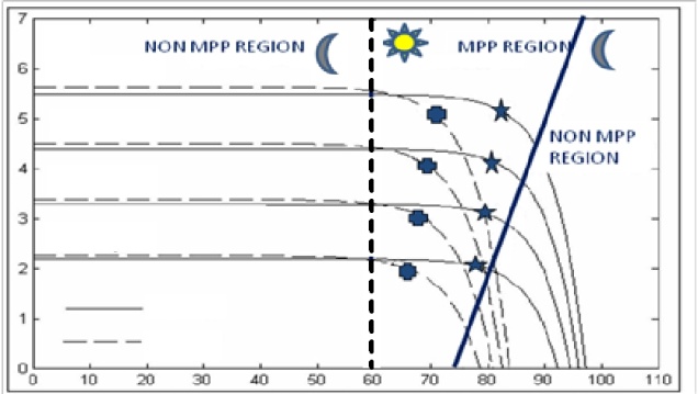 | Figure 1. PV array I x V characteristics and regions |
2.2. Variable ∆IPV and Non-Switching Zones Based on Fuzzy Logic
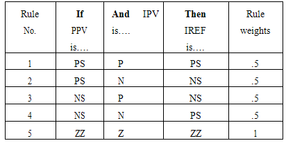
In order to improve the performance of the previous Scheme (1) under steady state conditions, one can use variable ∆Ipv-ref in the MPP region. In this case, since one knows that operation is close to the MPP, the range of the magnitudes of the variations of the reference current can be significantly reduced. The Fuzzy logic controller can be scaled down to model the operation of the system in the vicinity of the MPP only. New membership functions for the input and output variables and a new rule base (Table 1) were created for this case. The input variable ∆Ppv and the output variable ∆IPV-ref have 3 Fuzzy sets, and the rule base has 5 rules. In the non MPP regions, this scheme operates as Scheme 1 with the switch either fully ON or OFF.Table 1. Rule base for fuzzy model
 |
| |
|
3. Implementation of the Proposed Algonthm
3.1. Main Schematic Diagram for Non-Switching Zones and Fixed ∆Iref
The schematic diagram for this scheme is shown in fig 2. The PV output current ipv and voltage vpv are measured and multiplied for instantaneous PV output power ppv. The MPPT block processes vpv and ipv and outputs a current reference Iref. The PCC (peak current control) outputs the PWM driving signal. According to Iref and ipv, to the PC (power converter) block to make ipv follow Iref.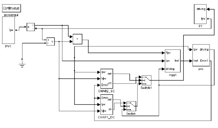 | Figure 2. Main simulation schematic for non-switching zones and fixed ∆Iref |
3.2. PV Panel
The PV panel simulation model is based on look-up table. This method is based on the model of the PV panel. The model of the PV panel is comprised of current source in parallel with a voltage source. In the classical PV cell, the input current decreases when the irradiation level falls. Likewise one can emulate a decrease in the sollar irradiation level by decreasing the current of the controlled current source [4]. The value of the PV output voltage is obtaind from a look-up table. So the simulation model of the PV panels used in the paper is shown in fig.3.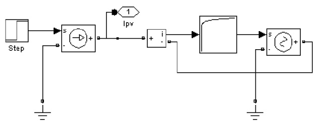 | Figure 3. Simulation schematic of PV panel |
3.3. Boost Converter
A boost DC-DC converter is used as the MPPT power converter in the PV system. Usually the output voltage of the converter is kept constant by the battery or another converter load. From the boost converter in fig.4 we know that VDS is zero when power switch SW is turned on, and is Vout when power switch is off. Therefore one can represent the power converter in the dashed line box is a controlled voltage source in series with a diode. When the gate signal of the power switch SW in fig.4 is “high”, the voltage VDS across SW is zero (MOSFET is on). In the simulation model, fig.5, CVS is controlled to output oV. On the other hand, if the gate signal is “low” VDS is equal to Vout (MOSFET is off). In the simulation model, fig.5, CVS is controlled to output 24V.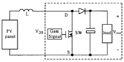 | Figure 4. Schematic of boost converter |
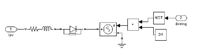 | Figure 5. Simulation schematic of boost converter |
3.4. MPPT Block
The MPPT algorithm is implemented in the MPPT block shown in fig.6. Samples of PV power PPV and PV current IPV are taken every switching cycle and the direction of perturbation of Iref is updated depending on the oprating point of the system on the PV VPV*IPV characteristic as determined by ∆PPV and ∆IPV. Additional Blocks such as the Short Circuit (SC) block and OPTION block, has been used to improve the oprating of the system under rapipidly changing atmospheric conditions. The SC block upon detection of a low value for VPV, send a signal to the MPPT algorithm to reduce Iref continousely and a signal to the PCC block to keep it oprating with minimum duty cycle. Otherwise, the PCC block would always oprate with maximum duty cycle, since IPV cannot reach Iref with VPV = 0V, this leading to a long transient with PPV = 0w. The OPTION block resets the value of Iref to the instantaneous value of IPV, when the diference between them exceeds a certain value. This block would usually come into effect during start-up and transient condition such as a large irradiance variation.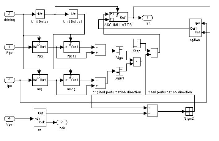 | Figure 6. Simulation schematic of MPPT block |
3.5. Peak Current Control Block
The schematic for the peak current control block is shown in fig.7. At the beginning of the each switching cycle , a short pulse from the Dmin block sets the output of the OR gate “1”, which goes to the gate driver circuit to turn on the power switch and make the inductor current to ramp up. It also unlocks and gate to permit the output of the comparator to go through it. At the beginning of each cycle, the actual current iPV is usually smaller than Iref and the output of the comparator is “1”. so even after output Dmin block changes from “1” to “0”, the output of OR will keep “1” until iPV and Iref match, or maybe iPV can not reach Iref in maximum duty ratio DMax, then Dmax block will output “0” to force the AND block to output “0” and the OR block to output “0”, turning off the power switch. So for the arrangement above the power switch will be on for at least DminTSW and at most DMAXTSW, during the minimum and maximum ON time interval, the switching off point depends on the relationship between Iref and iPV. When iPV reaches Iref the OR gate output “0”to turn off the power switch and lock the AND gate. Once the power switch turns off, it can not turn on again in the same cycle.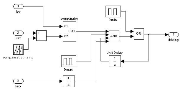 | Figure 7. Simulation schematic of PCC block |
In this scheme two blocks CHAR1_OC and CHAR2_SC are used to models the two curves as described above to demarcate the switching and non-switching zones.
3.6. CHAR1_OC
The CHAR1_OC block is shown in fig.8. The equation of the line that separates the MPP containing region and non-MPP containing zones corresponding to lower value of IPV then IMPP is implemented. VTO is obtained from the characteristic corresponding to the value IPV. Based on the comparison between VTO and VPV the switch will pass through the ON signal to keep the switch for D=1 or the output of the conventional peak current algorithm.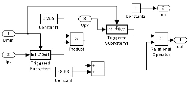 | Figure 8. Simulation schematic for CHAR1_OC |
3.7. CHAR2_SC
The CHAR2_SC block is shown in fig.9. The equation of the line that separate the MPP containing region and non-MPP containing zones corresponding to higher value of IPV then IMPP is implemented. VTs is obtained from the characteristic corresponding to the value IPV. Based on the comparison between VTs and VPV the switch will pass through the OFF signal to keep the switch for D=0 or the output of the switch corresponding to the CHAR1 _OC.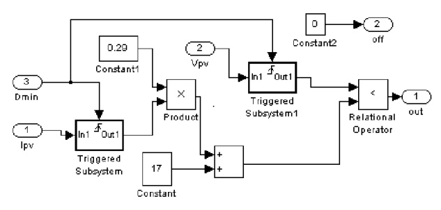 | Figure 9. Simulation schematic for CHAR2_SC |
3.8. Main Schematic Diagram for Non-Switching Zones and Fuzzy Controller
The schematic diagram for this scheme is shown in fig 10. The simulation schematic is the same as that used in the section 1.The Fuzzy logic controller (Fig. 11) is divided into four sections: Fuzzification Rule-Base, Inference and Defuzzification. The inputs to the Fuzzy logic controller are change in PV array power (Ppv) and change in PV array current (Ipv) and the output is the step change in converter reference current (Iref).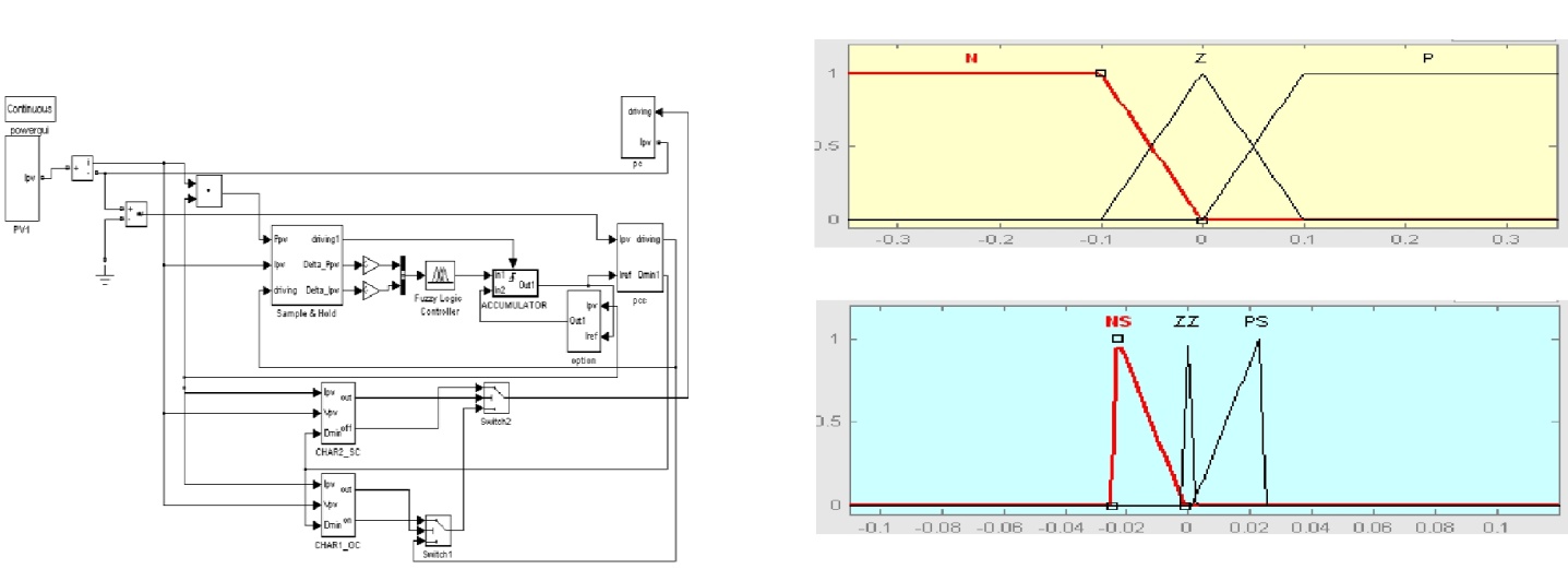 | Figure 10. Main simulation schematic for non-switching zones and fuzzy controller |
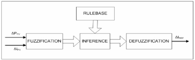 | Figure 11. Block Diagram of the Fuzzy controller |
Fuzzification and rule base is according to table 1 and fig.12 below. The Inference method determines the output of the Fuzzy controller. Mamdani's inference method has been used in our system. The output of the Fuzzy controller is a Fuzzy set. However a crisp output value is required. Hence the output of the Fuzzy controller should be defuzzified. The centroid method is one of the commonly used defuzzification methods and is the one we will employ for the proposed system. This method has good averaging properties and simulation results showed that it Function provided the best results.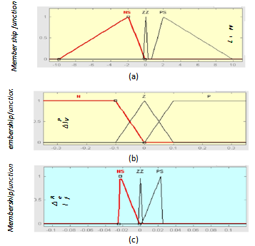 | Figure 12. Membership functions for the Fuzzy model; (a) Input PPV, (b) input IPV and (c) output IREF |
4. Simulation Results
Simulations were run in the Matlab/Simulink environment to verify the performance of the 2 schemes. The parameters are shown in the Appendix. Fig.13 shows the startup process under rated ambient conditions, the response to a step variation of solar irradiation to 50% of the initial value at 0.6ms and the response to the step-up of solar irradiation back to the rated solar irradiation at 1ms. For the simulation of the switching zone based schemes, the equations used for defining the regions in the Vpv x lpv plane are:Vpv = 0.255Ipv+18.63 and Vpv = 0.29Ipv+17It can be seen in Fig.13 that the non-switching zones based schemes present the fast rise time of 0.17 ms with both the fixed and variable ∆IPV ref because the converter operates with D =1. The Fuzzy logic based scheme presents a faster rise time.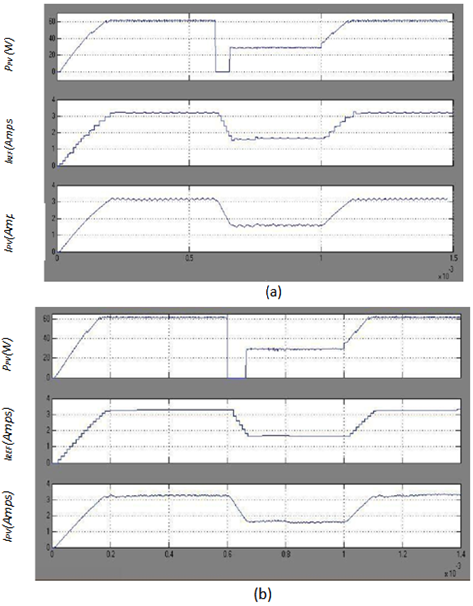 | Figure 13. Responses of the MPPT schemes (a) Fixed ∆lpv ref and nonswitching zones; (b) Fuzzy and non-switching zones |
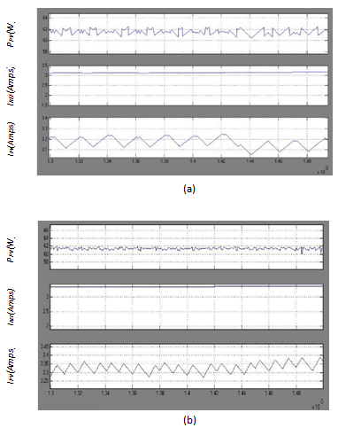 | Figure 14. Detailed steady-state (a) Fixed ∆lpv ref and nonswitching zones; (b) Fuzzy and non-switching zones |
5. Conclusions
This paper introduced the concept of non-switching zones in the Vpv x Ipv plane for implementing hybrid MPPT algorithms. By operating the power electronics converter with D equal to 0 or 1, depending on which non-MPP region the system operates, one pushes the operating point the fastest way possible towards the MPP region, where conventional P&O MPPT is used. Computer simulations show that this approach presents improved performance with respect to the conventional P&O MPPTs. The hybrid scheme allowed the use of smaller perturbations, reducing the power oscillation around the MPP and increasing the power yield in the steady-state without compromising the transient response. The use of variable size perturbations based on Fuzzy logic further reduced the power oscillations around the MPP.
Appendix
System Parameters
PV panel (at rated solar irradiation levels) Short-circuit current (ISC) = 3.452 A Current at the MPP (IMPP) = 3.29 A Voltage at the MPP (VMPP) = 18.62 V Open-circuit voltage (VOC) = 21.8 VBoost converterInductor (L) = 1 mHSwitching frequency (fsw) = 100 kHz Battery bankOutput voltage (VO) = 24 V
References
| [1] | X.J Liu and L.A.C. Lopes, “An Improved Perturbation and Observation Maximum Power Point Tracking Algorithm for PV Arrays,” Proceedings of the 35th IEEE Power Electronics Specialists Conference (PESC-04), Aachen Germany, 20-25 Jun. 2004, pp. 2005- 2010. |
| [2] | Neil S. D'Souza, Luiz A. C. Lopes and XueJun Liu, "An Intelligent Maximum Power Point Tracker using Peak Current Control," Proceedings of the 36th IEEE Power Electronics Specialists Conference (PESC-05), Recife, Brazil, 12- 16 Jun. 2005, pp. 172 - 177. |
| [3] | Hirotaka Koizumi and Kosuke Kurokawa, "A Novel Maximum Power Point Tracking Method for PV Module Integrated Converter," Proceedings of the 36th IEEE Power Electronics Specialists Conference (PESC-05), Recife, Brazil, 12-16 Jun. 2005, pp. 2081 - 2086. |
| [4] | Tsang, E.C.C.; Yeung, D.S.; Xi-Zhao Wang; “Learning weights of fuzzy production rules by a max-min neural network” Systems, Man, and Cybernetics, 2001 IEEE International Conference on; Volume 3, 7-10 Oct. 2001 Page(s):1485 – 1490. |
 Abstract
 Reference
 Full-Text PDF
 Full-text HTML