1. Introduction

In competitive market structures, such as centralized markets, standard auction markets, and spot-pricing or hybrid markets, the several studies have been published regarding the definition of a complete market model able to account for both economic and security aspects. Furthermore, the inclusion of the “correct” stability constraints and the determination of fair security prices have been properly addressed with so far so good. However, the inclusion of the FACTS devices for improving the techniques has not been addressed.

Reliability of the FACTS devices for enhancement the VSC-OPF performance included N-1 contingency criteria is focus of discussion in this paper. The hybrid markets and the two methods for the contingencies and stability constraints through the use of the VSC-OPF have been presented[1]. The OPF problem has been solved using an interior point method (IPM) that has proven to be robust and reliable for realistic size networks[2]. A proper representation of voltage stability constraints and maximum loading conditions, which may be associated with limit-induced bifurcations or saddle-node bifurcations, is used to represent the stability constraints in the OPF problem[3]. This technique has been applied to solve diverse OPF market problems as demonstrated in[1, 4].

Some studies for contingency planning and voltage security preventive control have been presented in[5], and the OPF computations with inclusion of voltage stability constraints and contingencies without installing the FACTS [1, 6] have also been discussed. However, the accounting of system contingencies in the VSC-OPF market problem with installing the FACTS has not arranged in the technical publication.

This paper uses the technique to account for system security through the use of voltage-stability-based constraints and the estimation of the system congestion through the value of the SATC as proposed in[1, 7] to OPF enhancement. In this case, voltage and power transfer limits are not computed off-line, which is the current common strategy, but are properly represented in on-line market computations by means of the inclusion of a loading parameter in the system stability constraints.

The following are some good proceedings for the FACTS applications and stability problems without discussion about placement of the FACTS devices. The effect of FACTS devices on the security re-dispatching have been presented by using the tool such as which provides a precise and quantitative analysis of OPF problems[8]. The other hand the methodology to ensure transient stability that relies on an OPF model with inclusion of transient stability constraints (TSC) in the OPF that based on the using of the concept of single machine equivalent (SIME) method and ensure transient stability of the system against major disturbances, e.g., faults and/or line outages[9]. Furthermore the incorporating the N-1 security criterion in order to reduce the size of the resulting OPF problem, a prior contingency filtering is used for reducing the size of the small-signal stability constrained OPF (SSSC-OPF) problem, where only incorporate contingencies that threaten system stability[10].

In this paper, the basic technique initially proposed in[11] and expanded in[1] with include contingencies, such that an accurate evaluation of the SATC can be obtained is further developed to include the FACTS devices, such that an enhancement the technique in[1] can be obtained.

The paper is organized as follows. Section 2 presents the mathematical model of the FACTS devices. Section 3 presents the basic concepts on which the methodologies are based that cited by means in[1] and advanced by applying the FACTS devices; the definitions of local marginal prices and nodal congestion prices and of SATC are also discussed by means of the literature in[1]. Furthermore in Section 3 discusses two techniques to account for contingencies in the OPF problem, with particular emphasis on their application to OPF-based electricity market models and then advances to allocate the FACTS devices. The applications of the proposed techniques are demonstrated in Section 4 for the IEEE 14-Bus test system assuming elastic demand bidding; for the test systems, results are compared with respect to solutions obtained with the standard OPF-based market technique without the FACTS and with the VSC-OPF based market technique included N-1 contingency criteria without the FACTS devices respectively. Finally, Section 5 resumes the conclusions as the main contributions of this paper as well as describes possible future research directions.

2. Mathematical Model of the FACTS Devices

Power Injection Model of the FACTS: The power-injected model is a good model for FACTS devices because it will handle them well in load flow computation problem. Since, this method will not destroy the existing impedance matrix Z; it would be easy while implementing in load flow programs. In fact, the injected power model is convenient and enough for power system with FACTS devices. The Mathematical models of the FACTS devices are developed mainly to perform the steady-state research. The SVC and TCSC are modeled using the power injection method[12] and UPFC [13].

2.1. The FACTS Devices

In an interconnected power system network, power flows obey the Kirchhoff’s laws. The resistance of the transmission line is small compared to the reactance. Also the transverse conductance is close to zero. The active power transmitted by a line between the buses and may be approximated by following relationships:

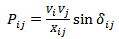(1)

or

where: and are voltages at buses i and j; : reactance of the line; : angle between the and . Under the normal operating condition for high voltage line the voltage and and is small. The active power flow coupled with and reactive power flow is linked with difference between the and . The control of acts on both active and reactive power flows. The different types of FACTS devices have been choose and locate optimally in order to control the power flows in the power system network. The SVC can be used to control the reactive power. The reactance of the line can be changed by the TCSC. The TCPAR varies the phase angle between the two terminal voltages. The UPFC is most power full and versatile device, which control line reactance, terminal voltage, and the phase angle between the buses. In this paper, three different typical FACTS are selected: SVC, TCSC and UPFC.

2.2. Mathematical Model of the SVC

Power Injection Model of the SVC: SVC can control bus voltage and inject reactive power, modelled by power injection model as example is effective to hold the voltage fluctuation in starting and stopping action of generator.

In this model, a total reactance is assumed and the following differential equation holds

The model is completed by the algebraic equation expressing the reactive power injected at the SVC node:

(3)

The regulator has an anti-windup limiter, thus the reactance is locked if one of its limits is reached and the first derivative is set to zero.

2.3. Mathematical Model of the TCSC

Power Injection Model of the TCSC: The algebraic equations of the basic TCSC structure with current control are:

(4)

where is the admittance of the line at which the TCSC is connected, and the indexes i and j stand for the sending and receiving bus indices, respectively.

The TCSC differential equations are as follows:

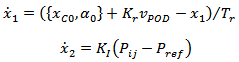(5)

where:

The state variables 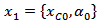depend on the TCSC model. The PI controller is enabled only for the constant power flow operation mode. The output signal is the series susceptance B of the TCSC, as:

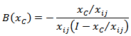During the power flow analysis the TCSC is modeled as a constant capacitive reactance that modifies the line reactance as follows:

where is the percentage of series compensation. The TCSC state variables are initialized after the power flow analysis as well as the reference power of the PI controller . At this step, a check of and/or anti-windup limits is performed. In case of limit violation a warning message is displayed. Initialization a check for SVC limits is performed.

2.4. Mathematical Model of the UPFC

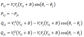
Power Injection Model of the UPFC: A series inserted voltage and phase angel of inserted voltage can model the effect of UPFC on network. The inserted voltage has a maximum magnitude of where the is rated voltage of the transmission line, where the UPFC is connected. It is connected to the system through two coupling transformers integrated into the model of the transmission line.

The whole UPFC model for representing power flow is depicted in Figure 1 or equation (6).

Figure 1. Complete injection model of UPFC

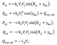(6)

Where: and : bus voltages, : equivalent series reactance, , : real power injection on bus-i, : real power injection on bus-j, : reactive power injection on bus-i, : reactive power injection on bus-j, : reactive power injection by converter shunt.

3. OPF Based Market Model

In[14] the standard-OPF based market model was presented. The OPF-based approach is typically formulated as a nonlinear constrained optimization problem, consisting of a scalar objective function and a set of technical limits such as equality and inequality constraints. The “standard” OPF-based market model can be represented using security constrained optimization problem[1].

3.1. Voltage Stability Constrained OPF

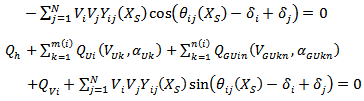
In the following, the security constrained OPF is modified and presented as proposed in[1], so that system security is modelled through the using in voltage stability conditions. Thus, as fundamentality, the VSC-OPF market model problems are:

Technical limits:

where and are vectors of supply and demand bids in dollars per megawatt hour, respectively; stand for the generator reactive powers; and represent the bus phasor voltages; and represent the power flowing through the lines in both directions, and are used to model system security by limiting the transmission line power flows, together with line current and thermal limits and bus voltage limits; and and represent bounded supply and demand power bids in megawatts. In this model, which is typically referred to as a security constrained OPF, and limits are obtained by means of off-line angle and/or voltage stability studies, based on an contingency criterion. Thus, taking out one line that realistically creates stability problems at a time, the maximum power transfer limits on the remaining lines are determined through angle and/or voltage stability analyses; the minimum of these various maximum limits for each line is then used as the limit for the corresponding OPF constraint. In practice[15], however, these limits are typically determined based mostly on power-flow-based voltage stability studies.

As this can see in[1], along with the current system equations that provides the operating point, a second set of power flow equations and constraints with a subscript c are introduced to represent the system at a maximum loading condition, which can be associated with any given system limit or a voltage stability condition. Equations are associated with a loading parameter (expressed in p.u.), which ensures that the system has the required margin of security. The loading margin is also included in the objective function through a properly scaled weighting factor to guarantee the required maximum loading conditions ( and to avoid affecting market solutions). This parameter is bounded within minimum and maximum limits, respectively, to ensure a minimum security margin in all operating conditions and to avoid “excessive” levels of security. Observe that the higher the value of , the more “congested” the solution for the system would be. An improper choice of may result in an unfeasible OPF problem if a voltage stability limit (collapse point) corresponding to a system singularity (saddle-node bifurcation) or a given system controller limit like generator reactive power limits (limit-induced bifurcation) is encountered.

3.2. Loading Parameter

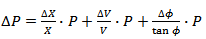
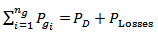
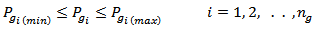
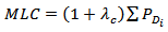
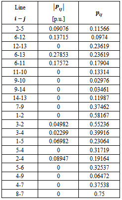
The economic dispatching is to minimize the overall generating cost , which is the function of plant output[24]

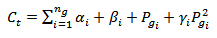(8)

Subject to the constraint that generation should equal total demand plus losses, i.e.

(9)

Satisfying the inequality constraints, expressed as follows:

However, the most accepted analytical tool used to investigate voltage collapse phenomena is the bifurcation theory, which is a general mathematical theory able to classify instabilities, studies the system behavior in the neighborhood of collapse or unstable points and gives quantitative information on remedial actions to avoid critical conditions[25]. In the bifurcation theory, it is assumed that system equations depend on a set of parameters together with state variables, as follows:

(10)

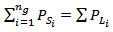
Then stability/instability properties are assessed varying “slowly” the parameters. In this paper, the parameter used to investigate system proximity to voltage collapse is the so called loading parameter , which modifies generator and load powers as follows:

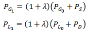(11)

Powers which multiply are called power directions. Equations (11) differ from the model typically used in continuation power flow analysis, i.e.

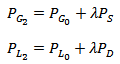(12)

where the loading parameter affects only variable powers and .

Thus, for the current and maximum loading conditions of (7), the generator and load powers are defined as follows[1]:

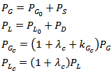(13)

where and stand for generator and load powers which are not part of the market bidding (e.g., must-run generators, inelastic loads), and represents a scalar variable used to distribute the system losses associated only with the solution of the critical power flow equations in proportion to the power injections obtained in the solution process (i.e., a standard distributed slack bus model is used). It is assumed that the losses corresponding to the maximum loading level defined by in equation (7) and equation (9) (8) are distributed among all generators; other possible mechanisms to handle increased losses could be implemented, but they are beyond the main interest of the present paper.

Therefore,

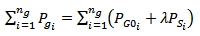(14)

and

(15)

And can be written as

(16)

Since the equation (14) becomes,

(17)

Furthermore, the can be minimized by the FACTS devices that installed at the best location in an optimal location), therefore will be maximizing the that will influence and increase power transfer or the power flow, because the level of loadability or the level of critical condition ( represents the maximum loadability of the network where this value viewed as the measure of the congestion of the network[16]) will be decreased. While, in the same manner for the demand can be arranged as

(18)

where will increase if is minimized by the FACTS.

3.3. Multi-Objective VSC-OPF with FACTS

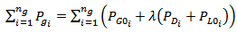
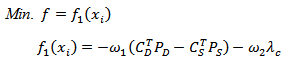
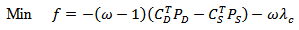
Furthermore, by modified the equation (1) as also in[16] the formulation of problem for Multi-Objective VSC-OPF with applying FACTS can be arranged as follows.

Objective function:

Equality constraints:

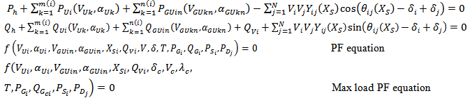Technical limits:

Inequality constraints:

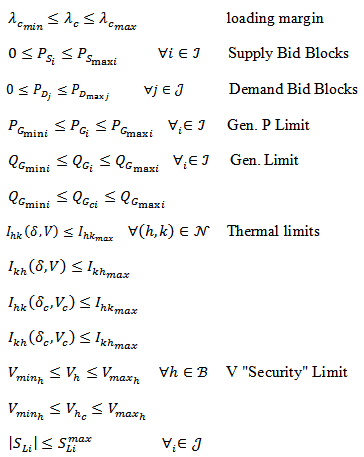Limit for the FACTS devices:

3.4. Local Marginal Prices and Nodal Congestion Prices

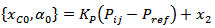
As presented in[1] and modified in this paper with allocated the FACTS devices, the solution of the OPF problem in equation (7) for without allocated the FACTS and equation (19) for allocated the FACTS provides the optimal operating point condition along with a set of Lagrangian multipliers and dual variables, which have been previously proposed as price indicators for OPF-based electricity markets. LMPs at each node are commonly associated with the Lagrangian multipliers of the power flow equations . These LMPs can be decomposed in several terms, typically associated with bidding costs and dual variables (shadow prices) of system constraints. From equation (7) and equation (13), the expressions for LMPs without FACTS obtained as.

where represents a constant load demand power factor angle.

The LMPs are directly related to the costs and , and do not directly depend on the weighting factor from the definition of equation (20). These LMPs have additional terms associated with which represent the added value of the proposed OPF technique. If a maximum value is imposed on the loading parameter, when the weighting factor reaches a value, say , at which , there is no need to solve other OPFs for , since the security level cannot increase any further[16], but in this paper as descript in equation (19), the security level can be enhanced with allocated the FACTS devices at a good location. Furthermore, if the FACTS are installed, the LMPs can be defined as

(21)

Where indicates Lagrangian multipliers of the power flow equations, stands for the dual-variables (shadow prices) for the corresponding bid blocks, which are assumed to be constant values. In (20), terms that depend on the loading parameter are not “standard”, and can be viewed as costs due to voltage stability constraints included in the power flow equations , while in (21), terms that depend on the loading parameter are steady-state, and can be viewed as costs due to voltage stability constraints included in the power flow equations . By using the decomposition formula for LMPs, equations (20) [1] and also equation (21) can be decomposed to determine NCPs that are correlated to transmission line limits and hence define prices associated with the maximum loading condition (MLC) or “system” available transfer capability (SATC).

where are the voltage phases and magnitudes , represents the inequality constraint functions (e.g. transmission line currents), and and are the shadow prices associated with the inequality constraints.

3.5. System Available Transfer Capability

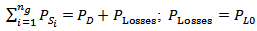
By using[1] the available transfer capability (ATC) concept is presented, as defined by NERC, is a “measure of the transfer capability remaining in the physical transmission network for further commercial activity over and above already committed uses”[17]. This basic concept is typically associated with “area” interchange limits used, for example, in markets for transmission rights. A “system-wide” available transfer capability is proposed to extend the ATC concept to a system domain[7], as follows:

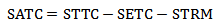(23)

Thus the for the VSC-OPF problem equation (7) and (19) can be defined as.

3.6. VSC-OPF Including N-1 Contingency

The solution of the VSC-OPF problem equation (7), equation (19) and the following equation (26) is used as the initial condition for the two techniques presented in here to account for a contingency criterion in electricity markets based on this type of OPF approach. Contingencies are included in equation (7), equation (19) and the following equation (26) by taking out the selected lines when formulating the “critical” power flow equations , thus ensuring that the current solution of the VSC-OPF problem is feasible also for the given contingency. Although one could solve one VSC-OPF for the outage of each line of the system, this would result in a lengthy process for realistic size networks. The techniques proposed in[1] address the problem of efficiently determining the contingencies which cause the worst effects on the system, i.e. the lowest SATC values that also is become the topic to discuss in this paper.

3.6.1. Iterative Method with Continuation Power Flow (CPF)

Considering N-1 Contingency Criterion

The flow chart of the method for including the contingency criterion, based on the continuation power flow analysis, in the VSC-OPF based market solutions depicted in in[1]. This method is basically composed of two basic steps, while in the block set supply and demand bids and as generator and loading directions is inserted the FACTS devices as dynamic component .

The VSC-OPF problem control variables, such as generator voltages and reactive powers can be modified by FACTS in order to minimize costs and maximize the loading margin for the given contingency because the OPF-based solution of the power flow equations and its associated SATC generally differ from the corresponding values obtained with the CPF, hence also needs an iterative process for the system installed FACTS.

It is necessary to consider the system effects of a line outage, in order to avoid unfeasible conditions when removing a line in equations , that it is other function of FACTS. For the given operating conditions, a line outage may cause the original grid to separate into two or more subsystems, i.e. islanding; where the smallest island may be discarded, or just consider the associated contingency as unfeasible.

3.6.2. Multi-Objective VSC-OPF with Contingency Ranking

This technique[1] starts with a basic VSC-OPF solution that does not consider contingencies so that sensitivities of power flows with respect to the loading parameter can be computed. Then, based on this solution and assuming a small variation of the loading parameter, normalized sensitivity factors can be approximately computed as follows:

where and are the sensitivity factor and the power flows of line , respectively; this requires an additional solution of for . The scaling is introduced for properly evaluating the “weight” of each line in the system, and thus considers only those lines characterized by both “significant” power transfers and high sensitivities[18].

3.6.3. VSC-OPF Market Model Including N-1 Contingency with FACTS Devices

The formulation of problem for VSC-OPF including N-1 contingency criteria where basically use equation (7) and equation (19) with allocating the FACTS devices can be arranged as follows.

Equality constraints:

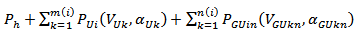
PF equation

Max load PF equation

Technical limits:

Inequality constraints:

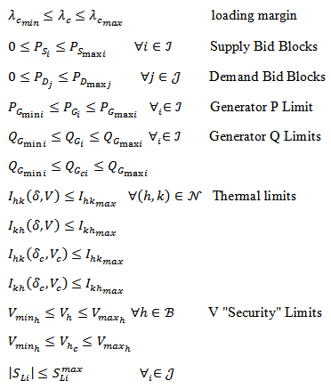where represent power flow equations for the system with under study with one line outage. Although one could solve one VSC-OPF problem for the outage of each line of the system, this would result in a lengthy process for realistic size networks. The techniques this paper address the problem of determining efficiently the contingencies which cause the worst effects on the system, i.e. the lowest loading margin and . The following is assumed to be defined using loading directions in equation (3.3) and then using equation (7.2) as presented in[19]:

where indicates the line outage, Observe that (27) analogy with equation (24), where the search for the minimum was limited only to the loading parameters. In equation (27) the minimum ALC is computed for the product of both and the TTL since power bids are not fixed and the optimization process adjusts both and in order to minimize the objective function. Finally, for a good case in FACTS installed the lowest loading margin and will be increase.

4. Example

The VSC-OPF problem in equations (8) and (17) and the techniques to account for contingencies are applied to the IEEE 14-Bus test system modified. All the results discussed here were obtained in Matlab[21] using the nonlinear predictor-corrector primal-dual interior-point method based on the Mehrotra’s predictor-corrector technique[20] where coded in the Power System Analysis Toolbox (PSAT)[22] and modified by the means of implementation of the VSC-OPF with N-1 contingency criteria installed the FACTS devices techniques. The results of the optimization technique in equation (7) are also discussed to observe the effect of the method on LMPs, NCPs and system security, which is represented here through the SATC. The power flow limits needed in equation (7) were obtained off-line, by means of a continuation power flow technique similar to the presented in[1]. For the test system, bid load and generator powers were used as the direction needed to obtain a maximum loading point and the associated power flows in the lines.

By using the same manner as the VSC-OPF with N-1 contingency criteria without installed the FACTS devices techniques[1], for the test case, the limits of the loading parameter were assumed to be and , i.e. it is assumed that the system can be securely loaded to an SATC between 10 and 80% of the total transaction level of the given solution. The weighting factor k in the objective function G of equation (8) and equation (17), used for maximizing the loading parameter, was set to , as this was determined to be a value that does not significantly affect the market solution. Furthermore, where had been found for the fixed value used to represents the is neglected , as this does not really affect results obtained with the equation (7) techniques[1] and the proposed techniques (equation (24)), since all computed values of SATC would be reduced by the same amount.

4.1. The 14-Bus Test Case

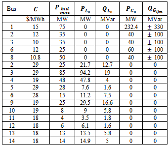
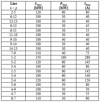
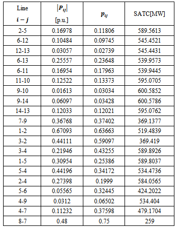
The IEEE 14-Bus test case, which is extracted from http://www.ee.washington.edu/research/pstca/ and then modified in this paper representing five generation companies (GENCOs) and eleven energy supply companies (ESCOs) that provide supply and demand bids, respectively.

In the Table 1 and Table 2, is proportional cost active power, is maximum power bid, is load active power, is load reactive power, is generator active power, is generator maximum and minimum reactive power, is line maximum apparent power limit, is line maximum active power limit, is line maximum current limit.

Table 1. GENCO and ESCO Bids Data for the 14-Bus

Table 2. Line Data for the 14-System

This section depicts the data set for the IEEE 14-bus test system. Table 1 shows supply and demand bids and the bus data for the market participants, whereas Table 2 shows the line data only for and . Maximum active power flow limits were computed off-line using a continuation power flow with generation and load directions based on the corresponding power bids, whereas thermal limits were assumed to be twice the values of the line currents at base load conditions for a variation kV voltage rating. In Table 2, it is assumed that 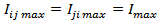and . Maximum and minimum voltage limits are considered to be 1.1 and 0.9 p.u, so that the results discussed here may also be readily reproduced as presented in[1].

4.2. Results and Discussion

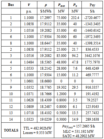
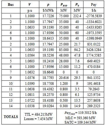
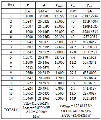
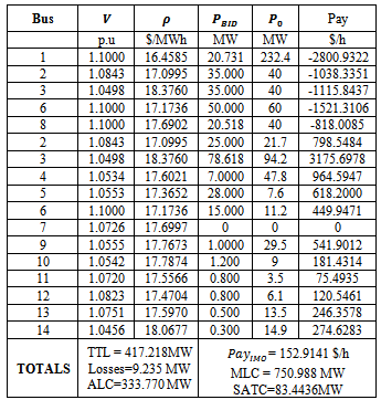
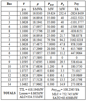
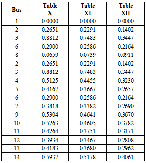
In the following for without and with installing the FACTS devices in Table 3, Table 4, Table 7, Table 8, Table 9, Table 10, Table 11 and Table 12, is voltage at each bus, is the LMP, is supply and demand maximum power bid, is generator and load active power including and , is pay for supply and demand. The other definition is the OPF-based approach which represents the maximum load-ability of the network. Furthermore, this value can be viewed as a measure of the congestion of the network, which is represented here using the following maximum loading condition (MLC) definition[19] in case before FACTS installed.

Table 3. OPF with Off-Line Power Flow Limit without FACTS

Table 4. VSC-OPF with Off-Line Power Flow Limit with UPFC on Line-11

Table 5. Sensitivity Coefficients       and SATC Determined Applying an N-1 Contingency Criterion without FACTS

(28)

Table 3 depicts the solution of equation (7), showing a low total transaction level (TTL) and the lowest SATC with respect to the maximum power limits of all bids, while as in case[1] the heterogeneous LMPs and NCPs also indicating that system constraints and in particular active power flow limits negatively affect the market solution, however can be corrected by applying FACTS. The SATC value, which was computed off-line with the continuation power flow, seems to be consistent with the chosen power flow limits. Table 3 depicts also the total losses and the payment given to the independent market operator, which is computed as the difference between demand and supply payments[1] as follows:

(29)

Table 4 depicts the results were be improved with allocated the UPFC in Line-11. The TTL, maximum loading condition (MLC), SATC, LMPs and voltages enhanced, while the total losses and given an enhancement.

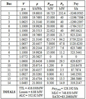
Table 6. Sensitivity Coefficients       Determined Applying an N-1 Contingency Criterion with UPFC

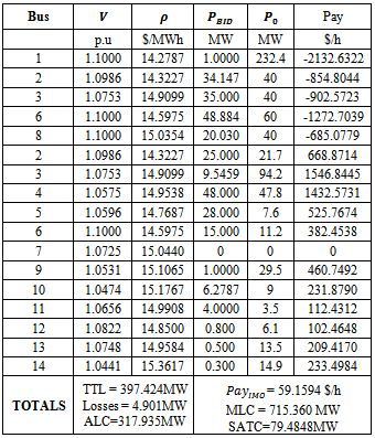
Table 5 shows the coefficients used for the sensitivity analysis and the SATCs computed by means of the continuation power flows technique for the two steps required by the iterative method described in Section 3.6.1 when applying the contingency criterion without installing the FACTS. Observe that both methods lead to similar conclusions, i.e. the sensitivity analysis indicates that the line 1-2 (Line-11) has the highest impact in the system power flows, therefore Line-11 becomes the best location of the FACTS devices, furthermore the contingency criteria show that the outage of line 1-2 leads to low SATC values. The line 3-2 has generation at the two ends and the line 7-9 has transformer with lower SATC value than the line 1-2, while the line 8-7 with lower SATC than those above, therefore leads to the lowest SATC values but do not use as the best location of the FACTS devices because also has transformer as described in[23].

Table 7. VSC-OPF with Contingency on Line 1-5 without FACTS

Table 8. VSC-OPF with Contingency on Line 2-4 without FACTS

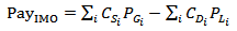
Table 6 shows the coefficients used for the sensitivity analysis when applying the contingency criterion which becomes decrease after installing the UPFC in line 1-2.

Table 9. VSC-OPF with Contingency on Line 3-2 without FACTS

Table 10. VSC-OPF with Contingency on Line 1-5 with UPFC on Line-11

Table 7, Table 8 and Table 9 as the following depict the VSC-OPF results for the critical line 1-5, line 2-4 and line 3-2 outage. This solution presents practically the same total transaction level as provided by the solution without contingencies in Table 3, but with different demand side bidding, and a higher SATC, as expected, since the system is now optimized for the given critical contingency. The rescheduling of demand bids results in slightly lower LMPs and NCPs, as a consequence of including more precise security constraints, which is also better results after installing the FACTS devices as seen in Table 10, Table 11 and Table 12 as the following, which in turn results in a lower value with respect to the one obtained with the standard OPF problem equation (7) in Table 3 (the higher losses are due the transaction level being higher). Furthermore Table 13 gives NCPs values about the topics that given in Table 3 until Table 12.

Table 11. VSC-OPF with Contingency on Line 2-4 with UPFC on Line-11

Figure 2 shows the system quiet stable after installing the UPFC on the Line-11 and gives the improvement for some parameter of the electricity base market.

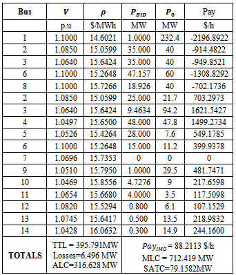
The SATC in Table 7, Table 8 and Table 9 corresponds to a , gives 20% of the total transaction level TTL, indicating that the current solution has the minimum required security level 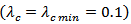with . As explained and expected without and with the FACTS, the higher minimum security margin leads to a lower TTL and, with respect to results reported in Table 7, Table 8 and Table 9, also LMPs and NCPs are generally lower, which is due to the lower level of congestion of the current solution. Observe that a more secure solution leads to lower costs, because the demand model is assumed to be elastic; hence, higher stability margins lead to less congested, i.e. lower, and “cheaper” optimal solutions. For the sake of comparison, Table 10, Table 11 and Table 12 depict the final solution obtained with allocating the UPFC in Line-11. In this case the whole results given satisfactory an enhancement or improvement.

Table 12. VSC-OPF with Contingency on Line 3-2 with UPFC on Line-11

Table 13. Nodal Congestion Prices Value ($/MWh)

Table 14. Nodal Congestion Prices Value ($/MWh) for System with UPFC on Line-11

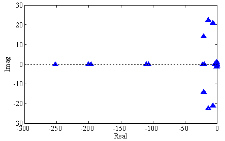Figure 2. Eigenvalue the IEEE 14-bus system with UPFC on line-11. Statistics of Eigenvalue: Positive eigs: 0; Negative eigs: 27; Complex pairs: 6; Zero eigs: 0; Dynamic order: 27

Finally, the found of a good system response for the allocated the FACTS devices indicates that the FACTS devices given a good response for the VSC-OPF method with presenting the security method (i.e., V "security" limits) and transaction method (i.e., power transfer limits) in equations (7), (19) and (26) which have the relationship to equation (1) and equation UPFC in Figure 2 for especially voltage, reactance and phase angle between the two terminal voltages.

5. Conclusions

The VSC-OPF based market enhancement are modified and tested on the IEEE 14-Bus test system. The results obtained with VSC-OPF based market including contingencies with installing the FACTS devices techniques and those obtained by means of the VSC-OPF based market including contingencies model only indicate that a proper representation of system security and a proper inclusion of contingencies with installing the FACTS devices, by using an allocation method, for the two result in improved transactions, higher security margins and lower prices.

The first method gave definition of the worst-case contingency by determining the lowest SATC with the off-line power flow limit without the FACTS as shown in Table 3 that can be improved with the FACTS as shown in Table 4, while the second approach computes sensitivity factors as indicated in Table 5 and Table 6 whose magnitude indicate which line outages and controlling of the FACTS devices maximally affect the system security and total transaction level as indicated in Table 7 until Table 12.

In the relationship with voltage, reactance and phase angle between the two terminal voltages on a transmission line, that is found a good system response for the allocated the FACTS devices which indicates that the FACTS devices given a powerful response for the VSC-OPF method with presenting the security method (i.e., voltage V "security" limits) and the transaction method (i.e., power transfer limits).

Further research work will concentrate in enhancement the OPF techniques performance with modifying of the model and control and then select the best variety and location of the FACTS devices.

ACKNOWLEDGEMENTS

The authors would like to thank for the support and helpful comments of academicals members Gadjah Mada University for this work.