1. Introduction

Few would deny the importance of electricity as an essential input to production and to economic activity in general. Based on the fact that changes in electricity prices impact on basically each and every person in South Africa, and more specifically on Eskom’s³ core business, it is important to determine its effect on each of these entities in South Africa.

Because South Africa has for long enjoyed low electricity tariffs, investors have previously been attracted to the electricity intensive sectors as a result of their price competitiveness. Low electricity prices compensated for other disadvantages such as volatile exchange rates and non-flexible labour[36, 27:27]. Consequently, a sustained boom developed in the mining and industrial sectors. This was in line with the South African government’s policy of the price of electricity was often lower than the cost of producing it, resulting in South Africa being known for its very low electricity prices around the world[25].

According to Van Heerden et al.[38:3], real electricity prices decreased significantly under the price compact announced in 1991. The main objective of decreasing the real price of electricity was to increase the South African economic growth rate. However, with the high economic growth levels obtained in later years, such as an economic growth rate of 5.6% in 2007, the utility started to face new challenges: higher electricity demand by customers, reserve margin problems, as well as capacity constraints[1:14]. Subsequently the country has experienced one of the most debilitating electricity crises of any emerging country in recent times, shutting down strategic economic sectors for days on end. The crisis is sustained in that the country’s state-owned electricity generator, Eskom, has requested industry to voluntary ration electricity consumption at 10 per cent less than historical levels of electricity demand for at least the next five years.

As demand for electricity began to near the available supply, Eskom found itself without financial provisions to react to the need for new generation capacity. As a result, discussions between the utility and the National Energy Regulator of South Africa (NERSA) resulted in significant electricity price increases. As a means of raising capital for the expansion, Eskom has been forced to look abroad for loans as well as to push up electricity costs to very high levels, the most recent of which are 24.8%, 25.8% and 25.9%increases to the tariffs for the years 2010 – 2012[27, 36]. Subsequently the 25.9% was reduced to 16% by NERSA[12].

The resulting lack of electricity supply / interruption of supply is increasingly recognised as a potentially serious constraint on sustained economic growth, the more so given the wide consensus on the important links between electricity and economic development⁴ (see e.g.[14, 5]).

Former Chairman of the Federal Reserve, Alan Greenspan, highlights in his memoirs that, while the amplitude of economic cycles seems to be decreasing, the frequency of cycles is increasing (differently put, the lag between increased and decreased economic growth cycles is shortening)[15]. This implies that businesses are facing changing economic conditions occurring more frequently, albeit the impact may be less pronounced (than e.g. in the first half of the 20th century). However, the challenge is that most of the major electricity consuming customers tend to have more “static” production processes in terms of technology, making them less “nimble” to adjust in short periods of economic fluctuation.

Eskom as a business (and the South African economy) is dependent on these major electricity consuming customers for electricity sales (and economic growth and employment). Total Eskom revenue⁵[11:330] relative to the South African national economy’s size amounts to approximately 2.6% of Gross Domestic Product (GDP6) (but approximately 1.7% when measured in gross value added contribution terms). For some further understanding it is important to contextualise these Key Industrial Customers (KICs). These accounts constitute more than 50% of total energy sold by Eskom on an annual basis and account for more than 40% of revenue (2010 financial year). In addition, this revenue is concentrated in approximately 150 accounts only.

• KICs revenue therefore amounts to approximately 1.1% compared to national GDP, which is significant.

• These approximately 150 accounts in turn are in sectors that directly account for a major share of economic output (21% of 2010 GDP at constant 2005 prices) as well as employment (15% of 2010 formal employment) of the South African economy. The industrial bias of these types of customers’ strong up- and downstream economic links implies that economy-wide output and employment will also significantly be affected due to changes in these sectors.

Within the above context, it is crucial for the utility (and policy makers and other stakeholders) to understand the impact of operational environment factors (e.g. changes in electricity supply pricing or availability) to these customers as well as their relationship with electricity consumption and potential financial risk implications to the utility (and the South African economy).

The aim of this paper is therefore to contribute towards developing a strategic information framework that can provide management with enhanced strategic decision making information regarding the context of KIC customers within the internal Eskom as well as the broader South African economy. In the current environment of dynamism around electricity prices and changing economic conditions the application of this framework will be to focus on the potential impact of increased electricity pricing for this paper, but in future will be expanded to also include other aspects of key customers’ business environments (e.g. impact of changes in the international markets and commodity prices and other relevant variables).

2. Approach

In light of the information presented in the introduction, the most pertinent question now is: how can or do producers position themselves in the present economic situation, while being aware of energy considerations, to avoid significant losses in profitability?

Some of the responses to higher electricity tariffs can include:

• Passing the cost onto the consumer or customer (except if the producer is a price taker e.g. some commodity suppliers, in which case international markets dictate price and it is nearly impossible to pass on costs);

• Initiating energy conservation or increasing use of alternative/self-generation of energy;

• Cutting costs in production and other areas (e.g. labour); and

• Reducing hours of production.

The level of demand and competition to a large extent determine how much of the rise in input cost (as a result of increased electricity prices) can be pushed over to the buyer. Changing the equipment used in the production process or building energy self-generation equipment in order to reduce production costs is often only done over a period of time and therefore will not necessarily reduce production costs in the short or medium term[19:25-28].

The increase in electricity prices may therefore result in lower price competitiveness in the short and medium term. For example, the steel industry has a very narrow profit margin. Most countries produce iron and steel domestically. Production for export is therefore limited during low price periods in order not to flood the market. Transalloys manganese-ore smelting in South Africa, for example, stopped operation for 2 months in 2009 due to lower current market demand[8].

However, at some point a decision can (or has to) be made to close down the operation, due to reaching a so-called “tipping point”. “Tipping point” events are often cited in the literature to explain the reasons why companies/industries would close down their operations due to non-economical operations (e.g. as a result of too high major input price levels).

Within the above context, it is crucial to understand the impact of operational environment factors (e.g. changes in electricity supply pricing or availability) to these customers as well as their relationship with electricity consumption and be able to link these relationships to the possible tipping points for key customers and potential implications thereof for the utility business and the economy.

By making use of the “tipping point” approach based on individual major customers and rolling these up into relevant sectors one can provide a basis for better informed decision making (as opposed to e.g. only a top-down economic sectoral approach), although this requires more effort in terms of information gathering and research and analysis. Combining the “tipping point” analysis implications as well as broader economic and socio-economic impacts serves to better inform the policy and management decisions in a more holistic way.

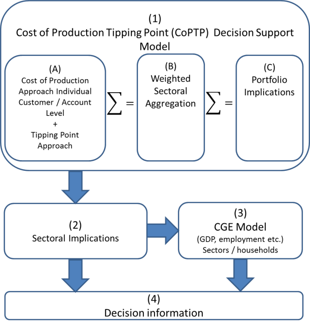Figure 1. High level modelling framework

Our approach needs to address the following elements identified to be relevant to this specific topic:

• Ability to model individual customer “tipping point” events linked to Cost of Production components;

• Ability to relate the implications to sectoral level; and

• Illustrate the potential implications on a portfolio level as well as for the national (macro) economy.

In order to achieve this we constructed a decision support modelling framework as illustrated in Figure 1. The framework consists of an analytical Cost of Production Tipping Point Decision Support model (1), of which the sectoral outcomes (2) is then used to inform assumptions for a Computable General Equilibrium (CGE) model (3) to produce an economy wide scenario to inform on various questions and decision making (4).

Next we discuss these elements briefly and bring together all the elements as illustrated in the high level modelling framework.

2.1. Combing a “Tipping Point” Approach and Cost of Production

The decision support modelling framework described in this paper therefore was constructed based on the concept of so-called “tipping point” events. We therefore refer to it as the Cost of Production Tipping Point Decision Support model (CoPTP-DSM) for brevity on the rest of the paper.

The opportunity cost (or “tipping point”) of continuing with production is assumed to be the interest rate that can be earned by lending or investing money holdings as opposed to continuing with production. Therefore, if the estimated gross profit margin for an account dips below this rate it is used as an indication of a “tipping point” event in the constructed model. The approach therefore requires two key pieces of information:

1) a reasonable proxy or measure against which the customer profit margin can be compared or tested, and

2) the cost of production contribution of the specific input (e.g. electricity).

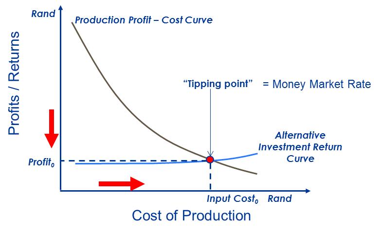Figure 2. Tipping point illustration

The “tipping point” graph (Figure 2) indicates that, as cost of production (via input costs) increase, the profit of the company concerned will decrease (all else constant). The money market rate⁷ is used for all the companies in this study as “tipping point” benchmark. Thus, as soon as profit declines to the level where the company concerned can earn just as much by the money market rate alone (Profit0, Input Cost0), the company will most likely close down operations (after a certain period of continued⁸ low profits or losses).

The CoP is determined by fixed and variable costs (regardless of changes in the activity level). In order to compare “like with like” across customers we need to exclude trade and transport margins required to move the produced end-product to the market. The reason for this can be explained through a numerical example.

Table 1. CoP Numerical Example Elements Customer A Customer B Average Fixed Cost 100.00 100.00 100.00 Input 1 Cost 20.00 20.00 20.00 Other Variable Costs 50.00 50.00 50.00 Cost of Production 170.00 170.00 170.00 Trade & Transport Margins 85.00 5.00 45.00 Other Sales Costs 20.00 20.00 20.00 Total Cost of Sales (Output) 275.00 195.00 235.00 Price 1.50 1.50 1.50 Units 200.00 200.00 200.00 Total Sales Value / Revenue (Price x Quantity) 300.00 300.00 300.00 Mark-up (Profit) 25.00 105.00 65.00 Profit Margin 8.33% 35.00% 21.67% Input 1 Cost as % of Total Cost of Sales (Output) 7.3% 10.3% 8.5% Input 1 Cost as % of Total Cost of Production 11.8% 11.8% 11.8% E.g. if Input 1 Increases e.g. 20% - profit impact Delta Input Cost 4.00 4.00 Delta Profit -4.00 -4.00 New Profit Margin 7.00% 33.67% %Change Impact on Profit Margin -16.0% -3.8%

Our example has two fictional customers (A and B). All cost elements are the same for the two accounts, except for the trade and transport margins as Customer A is further located from the market than Customer B.

The product and production processes are identical. If one therefore applies the high level approach of considering the contribution of input 1 (e.g. electricity) in this example, as a ratio of cost of sales (refer to this as case 1, as the typical calculation on which most sectoral comparisons based on Statistics South Africa [StatsSA] sectoral data are done), one would conclude that Customer A is less electricity intensive (as the cost of input 1 in this instance is 7.3% for Customer A as opposed to 10.3% for Customer B). A more accurate approach would be to exclude trade and transportation margins, as these are increasing the cost of sales and therefore increase the enumerator, resulting in a lower cost contribution of input 1 (refer to this as case 2).

A practical example would be customers exporting e.g. minerals to international markets versus domestic markets. The international delivery channel will add a major cost component to the cost of sales of output of the customer, while a customer with identical input cost contributions but a local market (and therefore relatively lower trade and transport margins) would not experience these additional costs. The end result would be that in case 1 Customer A (at 7.3%) would be interpreted to be less impacted by an increase of costs for input 1, while Customer B (at 10.3%) would be more impacted. In actual fact, both these customers are equally dependent on the specific input, but at different levels of profitability. All else constant, Customer A overall will be more negatively impacted than Customer B (profit margins for Customer A will decrease by 16% relative to only 3.8% for Customer B). However, an increase in electricity prices would possibly lead to other economy-wide price increases impacting the trade and transportation components as well, causing Customer A to be, relatively speaking, even further negatively impacted than Customer B (in terms of profit implications).

2.2. Collecting, Collating and Understanding the Data

The KIC internal account data was analysed to understand the specifics and relate to customer plant types, related energy usage and associated Eskom revenue. It was found that, although the KIC accounts number approximately 150, these accounts actually belong to between 60-70 individual companies, of which more than 55% are listed entities and 45%are private or parastatal (e.g. Transnet). In order to collect the make-up and contributions of major input costs for these companies a process of engaging these customers regarding the specifics of their production input costs (e.g. electricity, raw material, labour, imported cost contributions and others) was initiated. Due to the fact that this is highly confidential market intelligence, customers are extremely reluctant to provide such information and where provided is subject to confidentiality/non-disclosure agreements.

Total cost contributions of inputs obtained from clients accounted for 56% of the accounts, while another 14% could be derived from published financial and economic information. Sectoral average data published by StatsSA was applied for the remaining 30%. Financial (turnover and profitability) information applied was only available for approximately 3% of accounts directly from specific customers, while 13% could be derived from published annual report and economic data. The remaining 84% of accounts had to be estimated based on StatsSA published sectoral average data. Although the customer “sourced” information is not complete, it is a better starting point than just sectoral average data⁹. Currently approximately 70% of the KIC customer accounts are therefore relatively more accurately modelled than the “typical” economic sectoral average approach applied in most classic approaches.

When comparing aggregate sectoral averages, the reader must also be circumspect with the interpretation and application of information at sectoral level. It is best to use information at the most disaggregated level where possible, while at the same time also adjusting contributions as per the previous explanation regarding trade and transportation margins.

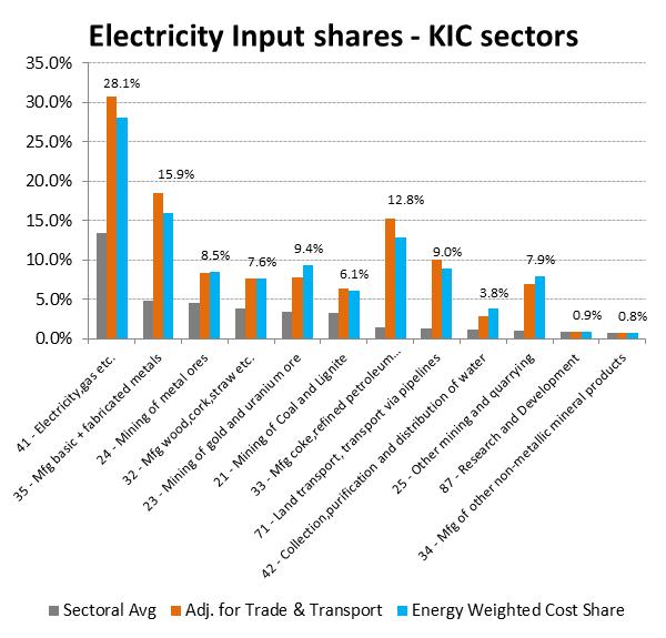Figure 3. Re-stated portfolio sectoral electricity input cost shares for key industrial accounts[32]

Furthermore, for the purposes of evaluating representation per Standard Industrial Classification (SIC) sector for the specific set of customers within the utility’s portfolio, these contributions were weighted by relative energy sales for a more representative sectoral (2 digit SIC) contributions picture for key industrial customers within the Eskom portfolio. Individual accounts are mapped to 5 digit SIC sectoral classifications. The difference in relative magnitudes for input cost contributions for KIC sectors is illustrated in Figure 3 (values for energy weighted cost contributions indicated).

When taking the same approach and information down to a specific customer (account) level, the picture can be much different for a specific customer – as indicated in Figure 4 where the individual accounts’ estimated electricity contributions of CoP are contrasted to the average electricity contributions of total intermediate output per sector (as per[32]). These contributions possibly may still understate the real electricity input cost contributions for a specific customer (unless directly obtained from the customer), but are much more realistic in order to inform decision making at a customer account level.

2.3. Constructing the Decision Support Modelling Framework

In order to help inform enhanced strategic decision making information regarding the context of KIC customers the CoPTP-DSM was expanded into a flexible decision support framework was developed in order to facilitate more timeous analysis of scenarios informed by changing economic and financial conditions.

The approach applied was to inform the analytical framework both from a macro-economic and sectoral perspective, combined with a “bottom-up” model comprised of first principle calculations, parameters and assumptions (for key customers).

A comparative static model was constructed to then inform outcomes against a “static” baseline informed by a forecast view for all variables as well as energy sales and revenue. The historical baseline for the model is calendar year 2010. Alternative scenarios, therefore, can be contrasted relative to such a baseline. The analytical framework was encapsulated in a Microsoft Excel © (Version 2007, 2010) interface to allow “what-if” and sensitivity analysis.

The benefits of this approach are that:

• In the event that (accurate) information for customers cannot be obtained, management is still in a position to inform decisions based on assumptions (ranges) and sensitivities;

• A process can be developed to improve coverage and accuracy of information used in a model over time;

• As key parameters change (e.g. commodity prices etc.) “fresh” analysis is possible at much reduced effort and time requirements;

• “Scenario” analysis can be conducted to inform management decisions;

• A logical, standardized and consistent (and repeatable) approach to inform relevant key questions is provided; and

• The framework becomes a “repository/reference” for quantified and systemized information regarding individual customers.

Some of the current critical questions that can be informed by this approach are:

• What are the various production input costs contributions of key customers?

• What is the energy intensity in each sector/industry?

• What are the customer bands within the same broader sectors?

• What will the potential effect be of price changes of input cost components on customers?

• What is the current gross profitability margin for a company or for a specific industry?

The initial application of this framework was to inform on the potential impact of increased electricity pricing.

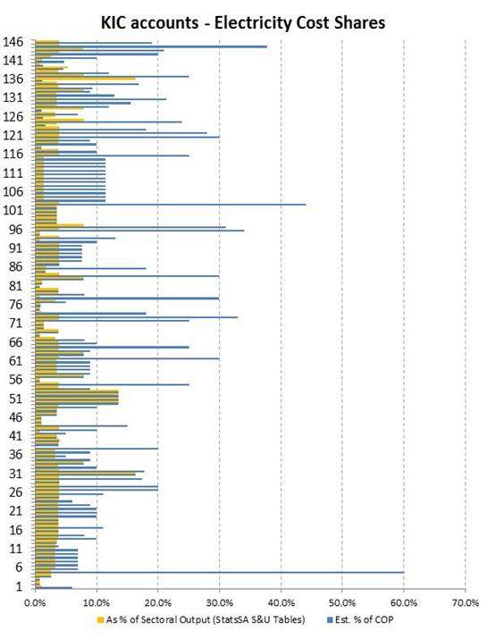Figure 4. Estimated electricity input cost shares for key industrial accounts[32]

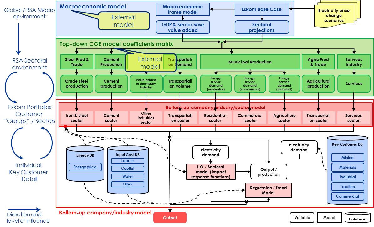Figure 5. The decision support modelling framework

3. Outcomes Obtained From Account Level Modelling

The actual outputs produced from the CoPTP-DSM decision support framework contain many different reports at individual customer account level that are also rolled-up into a sectoral and portfolio views. We provide some examples to give the reader a feel for what these outputs contain

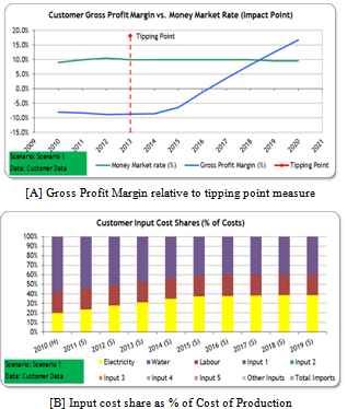Figure 6. Example account level outcomes

Figure 6 provides an example of output information for a specific client that experiences a “tipping point”.

Important to note from[A] in Figure 6 that for this specific customer the information gathering and modelling construction process already identified that this specific customer may be in jeopardy, even before applying any specific price increase scenario. If the customer can continue funding operations up to after 2017 it would seem that only then will the operation be profitable again. This fact was highlighted to the relevant stakeholders and subsequently in the first quarter of 2012 the “prediction”¹⁰ came true and the company publicly announced drastic cost reduction actions in order to remain sustainable. Although the specific account has not closed operations at the time of writing, such a probability exists subject to how economic and other parameters develop in the near future. Whether the account closes or not, the fact is that production and employment is affected and will be affected in future, and the approach and framework assist Eskom management with proactively flagging potential problematic accounts and help inform decision making around such accounts.

Figure 7 contains an example for a specific sector that will experience a “tipping point”.

On a portfolio level (grouping of 2 digit sectoral outcomes) some of the outputs for a specific year (2013) are illustrated in Table 2. Evident is that for this particular year the major concerning sector is SIC 35 – Manufacturing of basic and fabricated metals (containing e.g. Ferro manganese processing and Silicon metals processing).

A further illustration of implications over time is presented in Figure 8. The reference case excludes the pricing scenario, but includes the implications of the standard economic scenario assumptions used for Eskom planning purposes.

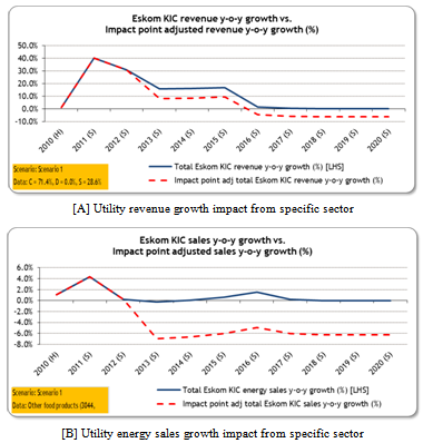Figure 7. Example sectoral level outcomes

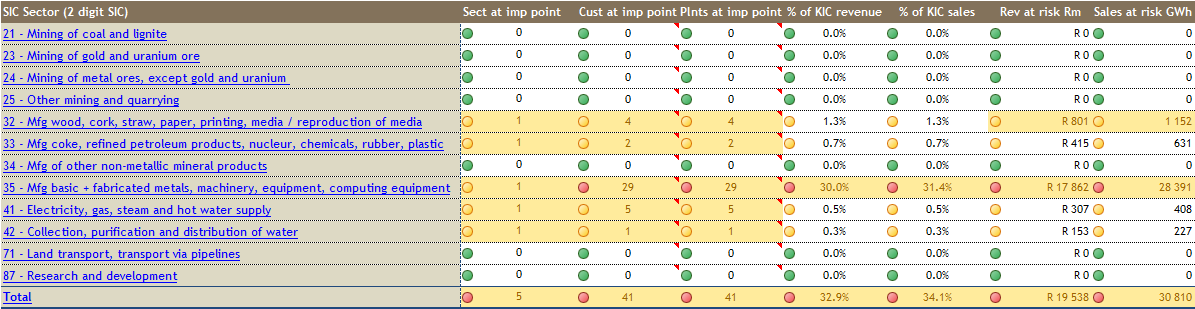Figure 8. Example portfolio level outcomes

Table 2. Illustrative Scenario Macro-Economic Implications (% Change)[* Exogenous by assumption] Annualised % Change Scenario: MYPD Price Impact – Key Customer Tipping Point Gross Domestic Product (GDP) -0.73 Employment -1.03 Average Real Wage Rate* 0.00 Domestic Consumption* 0.00 Consumer Price Index 1.66 Government Consumption* 0.00 Exports (Volume Index FOB) -1.79 Export Price Index 0.77 Imports (Volume Index CIF) 0.46 Import Price Index* 0.00 Balance of Trade (% of GDP) -0.50 Terms of Trade 0.77 Real Exchange Rate Depreciation/Appreciation -1.74

Figure 9. Example portfolio level outcomes

Evident from the graph is that based on the reference case economic scenario assumptions and specific assumption regarding the tipping point measure threshold,approximately 25 TWh per annum of energy (approximately 12% of total Eskom energy sold¹¹) is “at risk” or potentially susceptible to risk on a continuous basis due to economic developments and changes in the tipping point measure. Once the pricing scenario is applied (all else constant), this “energy at risk” increases to around 33 TWh per annum (to approximately 16%of total Eskom energy sold). So we can attribute the additional 4% energy at risk to the price increase (all else constant). From the analysis it was found that the manufacturing of basic and fabricated metals sector (SIC 35) contributes 92% to this additional energy at risk.

The following major outcomes resulted from the study regarding electricity price increase scenarios¹² (annual average price increase modelled at 25.8%[2011], 30%[2012], 16%[2013], 16% thereafter) for the specific set of customers for period 2012 to 2017:

• Overall 13 sectors (5-digit SIC) contain tipping point accounts accounting for approximately 25% of Eskom revenue with the most concentration in:

1) SIC 35 – Manufacturing of basic and fabricated metals (containing e.g. Ferro manganese processing and Silicon metals processing).

2) SIC 33 – Manufacturing of coke, refined petroleum products, nuclear, chemicals, rubber, and plastic.

• 9 accounts (6 customers) were flagged that clearly appear to potentially be in jeopardy based on the various tipping point analysis – accounting for 4.1% of the utility’s revenue and 3,623 GWh energy (4.0% in 2011 terms). Due to the confidential nature of this information and the fact that some of these companies are listed companies only the 5 digit SIC sectors to which these accounts belong are indicated in this paper. These are:

1) SIC 35111 – Conventional iron and steel (1 account)

2) SIC 35114 – Ferro manganese (1 account)

3) SIC 35225 – Zinc (1 account)

4) SIC 42000 – Collection, purification and distribution of water (2 accounts)

5) SIC 41300 – Steam and hot water supply (4 individual accounts)

• There are between 50 and 60 accounts experiencing at least one or more tipping point(s) over the period – but not on a sustained basis (this may however change as economic conditions or scenario assumptions applied in the model change).

4. Informing on the Broader Economic Implications

In the preceding sections we demonstrated an approach and framework developed to help enhanced strategic decision making information regarding the context of KIC customers. In this section we take this example further to illustrate how we can combine the first approach with the economy-wide modelling capabilities of an Applied General Equilibrium (AGE) model for South Africa.

In order to analyse the potential impact of the price increase scenario from the CoPTP-DSM in terms of the sectoral outcomes obtained we will use an Applied (or Computable) General Equilibrium (AGE) model of the South African economy. AGE models are the most appropriate tools to perform these types of analyses, and have been shown elsewhere to be particularly suitable for use in modelling energy-related issues. Bhattacharyya[4] provides an overview of AGE models that have been applied to improve the understanding of energy policy implications in various countries such as Australia, Sweden, Norway, Belgium, the United States, the Philippines and various applications to the global economy over the period 1974 to 1993. Subsequently many more such models have been developed and applied since 1993 on topics ranging from carbon emission tax policies (e.g.[35]) toanalysing the impact of stimulus to energy efficiency on the economy and environment (e.g.[16]).

In South Africa AGE models have also been used with increasing frequency since it was first used in the country by Naudé and Brixen[21]. Initially AGE models in South Africa were mainly used to analyse trade issues (e.g.[7, 23, 24]) and later to study labour market issues, environmental impacts, the impact of HIV/AIDS and fiscal issues, amongst others (see e.g.[2]). Energy issues however, have not yet been a major area of focus in the growing application of AGE’s. At the time of writing we were aware of a few formal studies into energy issues using an AGE model in South Africa namely by Altman et al.[1], Cameron and Naudé[6], Van Heerden et al.[37] and De Wet and Van Heerden[10] – the third and last of these concentrated on energy-environment interactions and not on supply and price shocks in the sector, while the first and second specifically focused on supply shocks as a result of the 2008 electricity load shedding experienced in South Africa. Our search was not exhaustive and we are aware that after the 2008 crisis energy issues have started receiving a lot more focus.

Thus, a further contribution of our paper is to extend the application of AGE modelling in South Africa in the context of energy issues, but the focus being that of major energy consumers and the potential implications of electricity price increases on individual customers as well as the resulting potential economy-wide effects.

4.1. Constructing the Key Customer Tipping Point Pricing Scenario

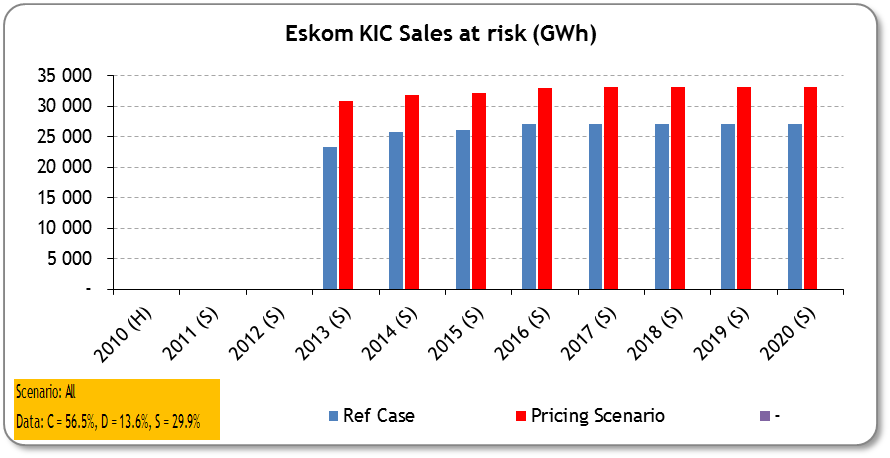
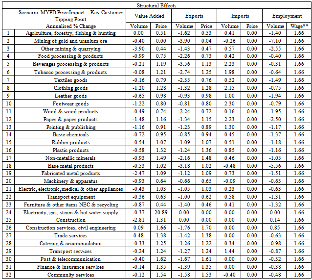
Due to the fact that the AGE model only contains 2 digits SIC sectoral detail, we aggregate the outcomes from the CoPTP-DSM to 2 digit sectors for modelling purposes. For analysis purposes we assume that the specific customers (3) contributing to the increase in energy at risk will actually close their doors and halt production. For this purpose we model only the impact of the potential loss of 3.7% of energy demand¹³ from the manufacturing of basic and fabricated metals sector (SIC 35) represented by model sector 19 (Fabricated metal products). The simulation we construct therefore models an impact on the national economy of reducing the intermediate demand for electricity (model sector 24) by the AGE manufacturing of basic and fabricated metals sector (model sector 19) translating into an intermediate electricity demand reduction of 2.8% per annum for this specific sector (refer to appendix A – section A.3 for more details).

The national level impacts of the simulations arepresented in Table 3. This illustrative analysis mainly focuses on two variables, that of overall economic output measured by Gross Domestic Product (GDP) and employment. Theresults are presented in annualised percentage change format.

The cause-effect logic of the simulation would be that as a result of the fact that these specific firms close down their operations, other sectors loose sales / production output as a result of the up-and down-stream linkages, as well as consumer demand reduction due to induced employment losses. For sectors such as mining and base metals the impact is more significant than other sectors, with relatively larger implications for employment in these sectors (refer to Table 4). The construction sectors are less impacted.

Table 3. Illustrative Scenario Macro-Economic Implications (% Change)[* Exogenous by assumption] Annualised % Change Scenario: MYPD Price Impact – Key Customer Tipping Point Gross Domestic Product (GDP) -0.73 Employment -1.03 Average Real Wage Rate* 0.00 Domestic Consumption* 0.00 Consumer Price Index 1.66 Government Consumption* 0.00 Exports (Volume Index FOB) -1.79 Export Price Index 0.77 Imports (Volume Index CIF) 0.46 Import Price Index* 0.00 Balance of Trade (% of GDP) -0.50 Terms of Trade 0.77 Real Exchange Rate Depreciation/Appreciation -1.74

Table 4. Scenario Illustrative Sectoral Implications (% Change)[* Exogenous by assumption] [** Nominal]

In general the effect is relatively small and for scenario (A) at 0.73 per cent lower GDP and 1.03 per cent lower for employment, compared to the base case in a comparative static fashion (for a review of the interpretation of thesetypes of comparative static results refer to Horridge et al.[17]).

For more context, if we translate this in terms of GDP growth and constant 2005 GDP monetary value it would yield approximately R13.8 billion relative to 2011 real GDP[28] for South Africa (R 1,895.7 billion x 0.73/100). In terms of forward looking growth this can be interpreted that if South Africa targets 3 per cent growth for a given year, the impact of this scenario would result in the economy only realising 2.3 per cent growth. In terms of employment context (non-agricultural sector employment) this would translate into approximately 86,304 employment positions lost for South Africa (8,379,000 x 1.03/100)[34].

The result is that production volumes decline while price need to adjust upwards to compensate. The price increase implies a contraction of exports so that the equality between the given world prices and the marginal costs of export supplies is restored in all industries. Domestic supply will also decrease because the prices of domestic products relative to the import prices increase (imported prices assumed constant) and import volumes will increase as a result. Total production therefore declines and is propagated through the inter-industry input-output linkages. Overall domestic consumption is assumed fixed (but will change on income group level) and the resulting general domestic price increase that needs to take place to achieve equilibrium is approximately 1.7 per cent, while the imported price index stays constant as South Africa is assumed to be a price taker in the international market. Import volumes continue to increase at 0.46 per cent as a result of the South African economy’s high import propensity.

Since producers are assumed to maximise profits, employment loss is the result of reduced outputs combined with sticky (and even increasing) wage rates (average real wages assumed fixed). The employment loss in turn leads to a smaller wage bill being paid to labour, with the resulting feedback of declining household income.

We present some sectoral outcomes in Table 4. Although most sectors are negatively impacted, most notably (and as expected) the mining industries, base metal and fabricated metals (itself) bears the brunt of the impact. Employment losses range from 1.5% to 7% for these four sectors.

Table 5 presents the distributional results of the scenario in terms of changes in real household consumption and the corresponding changes in household-specificconsumption-price indices. Overall the group that is affected the most negatively by the increase in electricity prices are the lower income groups across all race groups. This is to be expected as employment in the mining and manufacturing sectors are most adversely affected.

These outcomes for GDP and employment compares well with the outcomes obtained in one of the most comprehensive studies on this type of topic in recent years conducted by Altman et al.[1]. For the Altman et al.[1] 2B scenario (rationing mining and smelters by 4.3%) the outcome obtained was a 1.1% annualised decrease in real GDP and -1.5% for employment (Table 2, Altman et al.[1:26]). Although the impact obtained in this analysis was relatively less negative (0.73 % annualised decrease in real GDP and -1.03% for employment) we must keep in mind that we make a very different and conservative assumptions in the context of assuming that these large customers in the basic metals fabrication sector would actually halt production overall, and no direct implicationsfor the mining industry are assumed. The knock-on effect of the complete ceasing of production activities in these three customers have potentially much wider-ranging impactsthan that of only a partial reduction in electricity consumption/demand as illustrated by the scenario.

The results serve to illustrate how different the implications of the outcome of the scenario can impact the national economy depending on which economic agents have to bear the brunt of the effect of the specific question being modelled.

Table 5. Distributional Results for Households

5. Summary

The outcomes obtained from the “direct” analytical Cost of Production Tipping Point Decision Support model (CoPTP-DSM) describing how we can model on an individual customer level, rolled up to sectoral and portfolio level have been demonstrated. By translating outcomes for individual customers via sectoral aggregation we have demonstrated how the economy-wide implications can be informed by combining this approach with that of an Applied General Equilibrium model.

The following major outcomes resulted from the CoPTP-DSM electricity price increase scenarios (annual average price increase modelled at 25.8%[2011], 30%[2012], 16%[2013], 16% thereafter) for the specific set of customers for period 2012 to 2017:

• Overall 13 sectors (5-digit SIC) contain tipping point accounts accounting for approximately 25% of Eskom revenue with the most concentration in:

SIC 35 – Manufacturing of basic and fabricated metals (containing e.g. Ferro manganese processing and Silicon metals processing).

SIC 33 – Manufacturing of coke, refined petroleum products, nuclear, chemicals, rubber, and plastic.

• 9 accounts (6 customers) were flagged that clearly appear to potentially be in jeopardy based on the various tipping point analysis - accounting for 4.1% of the utility’s revenue and 3,623 GWh energy (4.0% in 2011 terms).

We modelled the economy-wide impact of a scenario where we assumed 3 major customers14 identified with the CoPTP-DSM will close operations as a result of the price increases. The effects on GDP and employment results in a 0.73 per cent lower real GDP growth and 1.03 per cent reduction in overall employment when compared to the base case.

When comparing our outcomes with another recent study of similar nature (that of Altman et.al.[1]) we have found that while the approach and dynamics assumed in framing the questions and approach were different, the relative outcomes of these studies support each other.

We propose that while more and better informed decisions can be made by making use of such a decision support framework (combining large customer specific cost of production “tipping point” models and pure economic AGE models) to inform both policy and strategic and tactical business decision making, focused effort on obtaining relevant information to apply in such models is required.

6. Conclusions

In conclusion it must be kept in mind that there are factors that our approach currently does not account for in these scenarios or to which the model is quite sensitive:

• Overall – the level of the specific “tipping point” measure assumption (in this instance money market rate);

• The CoPTP-DSM is sensitive to exogenous variables regarding future projected energy sales, exchange rates, interest rates and commodity prices;

• Other cost escalations (e.g. other major inputs like labour costs, other primary inputs);

• Second round economic effects (such as increased inflation as a result of production cost inputs and possible lower economic growth as a result) is not currently explicitly modelled;

• The CoPTP-DSM cannot account for management style and the ability to optimise/turn around a specific business and achieve cost containments in innovative ways; and

• Lastly, the CoPTP-DSM also cannot account for the willingness and depth of shareholders in terms of financial resources as well as medium to longer term strategy and views – when to get out of the specific business or when to continue until the market turns.

Information and estimates of cost contributions for specific customers are in the process of being improved, as well as the model itself. Therefore outcomes from the model will change / improve over time. This process will allow for more scenario-based decision information around potential implications of various changes in the operational environment of key industrial customers. Due to the fact that such a logical, standardized and consistent (and repeatable) approach to inform relevant key questions has been created, it is envisaged that the framework will become part of the division’s market intelligence and decision information process and will be a repository for quantified and systemized information into the future. While the application of this framework was focused on illustrating the potential impact of increased electricity pricing for this paper, it will be expanded to also include other aspects of key customers’ business environments (e.g. impact of changes in the international markets and commodity prices and other relevant variables) in the future.

We propose the following recommendations to the regulator in the context of the question i.e. how can South Africa’s economic regulators contribute to cost-effective delivery of essential infrastructure in the face of key financial, social and environmental pressure?

• The first recommendation is obviously to make use of these types of tools and analysis to inform policy and related debate and questions.

• In order to be in a position to have such models data (and quality of data) is imperative and the regulator need to ensure that all relevant stakeholders (utility providers such as Eskom and the municipalities) monitor, collect and report relevant and quality information to enable informed decision making.

• We also propose that the regulator require utility providers to demonstrate how the application of such frameworks and models were applied to inform key decisions – to ensure thorough systems-level thinking was applied to inform decisions.

• In order to enable utility providers to obtain and be able to use relevant information, the regulator needs to engage with other relevant stakeholders such as the Departments of Energy, Public Enterprise, Trade and Industry, Cooperative Governance and Traditional Affairs15, the Competition Commission and Statistics South Africa to facilitate collection and access to relevant information for utility decision making purposes.

By no means do we propose to have all the answers, nor were the illustrative scenarios in this paper aimed to inform on the value of a specific parameter or issue. The overall paper needs to be interpreted in the context of the aforementioned question and the illustrative nature and value derived as such, rather than specific answers or estimates of impacts and variables.

ACKNOWLEDGEMENTS

The authors are grateful for the helpful comments of the participants to the first South African Economic Regulators Conference, Johannesburg, 21 – 22 August 2012. Helpful discussions at the conference and also with Eskom have informed this paper.

APPENDICES

A. Appendix A – AGE Modelling Definitions, Model, Closure Rules and Assumptions

A.1. Definition And Concept of Age Modelling

AGE methodology is fairly widely known and many useful descriptions exist. We will therefore not provide any detail on this modelling methodology, but rather a high level summary and refer the reader to further descriptions in Cameron and Naudé[6], Naudé and Coetzee[23] and Naudé and Rossouw[24] who use similar methodologies. Rather than referring the reader to other papers, we replicate (with permission) parts of Cameron and Naudé[6] to facilitate context for the reader in this paper in sections of this appendix.

An AGE model can be defined as ‘an economy-wide model that includes feedback between demand, income and production structure, and where all prices adjust until decisions made in production are consistent with decisions made in demand’[9:132]. A typical AGE model has a theoretical structure that consists of a set of simultaneous equations describing, for some time period:

• Producers’ demands for produced inputs and primary factors;

• Producers’ supplies of commodities;

• demands for inputs to capital formation;

• household demands;

• export demands;

• government demands;

• the relationship of basic values to production costs and to purchasers’ prices;

• market-clearing conditions for commodities and primary factors; and

• numerous macroeconomic variables and price indices.

Demand and supply equations for private-sector agents are derived from the solutions to the optimisation problems (cost minimisation and utility maximisation) which are assumed to underlie the behaviour of the agents in conventional neoclassical microeconomics. Producers select inputs in order to minimise costs of a given output subject to non-increasing returns to scale industry production functions. At the same time consumers are assumed to select purchases in order to maximise utility functions subject to their budget constraints. Production factors are paid according to their marginal productivity. The government sector is included and imperfect competition can be introduced via price fixing, rationing and quantitative restrictions. At the equilibrium level these models’ solutions provide a set of prices that ensures that all commodity and factor markets are cleared as well as making all individual agents’ optimisations feasible and mutually consistent[3:12].

AGE models share three common features, the first being that they focus on the real side of the economy. Second, their supply and demand functions explicitly reflect the behaviour of profit maximising producers and utility maximising consumers. Third, both quantities and relative prices endogenous to these models, as well as the resource allocation patterns determined by them, have their roots in the Walrasian general equilibrium[40:8]. These features make them particularly suitable to model the role and impact of energy in the economy¹⁶.

The model is applied (or computed) using economy-wide consistent data on a particular economy as is normally contained in a Social Accounting Matrix (SAM)¹⁷ In the present case we use the 2002 published SAM¹⁸ for South Africa[30]. The SAM provides information to calibrate the majority of the parameters in the model. Other parameters, in particular expenditure elasticities¹⁹ are obtained from outside the model (typically from econometric studies or by making plausible guesstimates). The system of equations is solved so that the original SAM database is obtained as a solution to the system of equations. Simulations are now carried out by changing parameter values or exogenous variables and solving the model to obtain a new SAM as solution. By comparing the new SAM with the original SAM database will indicate the extent of changes implied by the policy or shock that was simulated. Thus, AGE analyses are mostly comparative static in nature, comparing different equilibrium positions associated with policy changes or shocks. AGE models are often made dynamic, albeit in a crude fashion, through specification of an endogenous investment function. They are also sometimes linked to a micro-simulation model which is based on a household survey so as to analyse in greater detail the poverty dynamics of economy-wide changes[23].

In the following section we describe the specific model which we will use in the case of South Africa.

A.2. AGE Modelling Framework – Adapted UPGEM

In this paper we use a South African adaptation of ORANI-G²⁰ to solve the model. It is known as the ‘UPGEM’ and was developed for South Africa by the University of Pretoria with the assistance of Centre of Policy Studies and the Impact Project from Monash University, Australia (see e.g. http://www.monash.edu.au/policy/orani- g.htm). The UPGEM model used in these simulations distinguishes 32 sectors, 6 household types and 4 ethnic groups[18]. For a more detailed exposition of the general modelling approach followed in UPGEM, see Horridge et al.[17]. A recent application of the model is contained in Van Heerden et al.[37].

For present purposes we adapted the UPGEM and the underlying dataset in the following manner:

First, we provided our own empirically estimated ‘Armington’ elasticities (intermediate, investment and household) based on Naudé et al.[22]. The standard UPGEM model use assumed elasticities based on those of the Australian ORANI model.

Second we made a number of adjustments to the way in which the gold mining sector is modelled. The gold mining industry (industry 2 in UPGEM) includes the extraction of gold ore and its refinement. For heuristic purposes, the output of the industry can be thought of as ‘ounces of refined gold’ not ‘tons of gold ore’. With the exception of a small amount sold to the domestic jewellery industry, the bulk of the country’s gold output is exported. The specification introduced to the UPGEM recognizes that in the short run employment in the gold industry and the amount of ore extracted is unresponsive to variations in the Rand gold price net of ore-extraction and refining costs.It also recognizes that industry policy is to vary the quality of the ore extracted with the net gold price.That is, if the net price rises (falls), lower gold yielding (higher gold yielding) ore is mined, resulting in an approximately constant profitability of the extraction/refining process.There is therefore a negative short-run relationship between the net gold price and the output of refined gold in the model.This is achieved through:

• an equation linking the percentage changes in the rental rate on the industry’s capital and the average wage which it pays for labour; and

• endogenising the industry’s all-input-using rate of technical change.

• Setting the export-demand elasticity for gold at -100 in order to ensure that variations in export volumes will have no effect on the foreign-currency gold price.

The current definition for the electricity sector as contained in the model equations and database includes the broad SIC[29] division 4 – Electricity, gas and water supply. This sector includes the following activities: the production, collection and distribution of electricity (SIC411), the manufacture of gas; distribution of gaseous fuels through mains (SIC412), steam and hot water supply (SIC413) and the collection, purification and distribution of water (SIC420). For the purposes of analysing the effects of changes to the electricity sector the ideal would have been to further refine the model and database to isolate the electricity sector (SIC411) from the other sectors. However, due to time and resource constraints this was not attempted for the purposes of this paper. An approximation approach was used based on the Supply and Use tables[30] to scale shocks and results with the relative contribution of the products SP139 – electricity, gas, steam and hot water supply(containing SIC411 to SIC413) and SP140 – collection, purification and distribution of water (containing SIC420). The structure of the model also therefore implicitly does not currently allow for switching of energy technologies.

A.3. Scenario’s – Closure Rules and Other Assumptions

The concept of‘closure rules’ refers to the way in which the number of endogenous variables in a model is set equal to the number of equations of the model in order to ensure that there will be a mathematical solution to the system of equations (or model)[26, 39]. Different closures for the same model will change the model’s quantitative characteristics, and it is therefore important to apply the correct closure depending on the specific question being analysed[3:17].

The general closure assumptions for the illustrative short-run comparative-static simulations conducted are:

• the numeraire is the world average price of all goods;

• capital stock is assumed fixed in each industry;

• no relative change in government consumption expenditure is assumed;

• slack labour markets for all labour categories are assumed;

• average real wages are kept constant – so wage rates adjust with inflation;

• household consumption moves with disposable income for all households; and

• the industrial structure of private investment responds to changes in relative rates of return.

In the short-run closure applied for this analysis, wages do not adjust in the labour market. It is assumed that real wage is fixed and total investment, total consumption and total government demand are also assumed to be fixed. Compared to the standard closure[17], real household consumption ‘x3tot’ is exogenous instead of total nominal supernumerary household expenditure ‘w3lux’. This implies that the aggregate level of household consumption is fixed. Aggregate real investment expenditure ‘x2tot_i’ is exogenous instead of the economy-wide rate of return ‘invslack’. This means that the level of investment is fixed. Aggregate real government demands ‘x5tot’ is exogenous instead of shift parameter ‘f5tot2’. Consequently, net export is the only demand changing endogenously.

For the specific scenario we have to make certain industry-specific assumptions over and above the general closure described above. We therefore have to assume that:

• electricity under these circumstance will not be exported – we know this in practice not to be the case, but the current treatment of the electricity industry in the model’s database assumes no imports or exports for the sector21; and

• employment in the electricity sector will not be shed in reaction to the decline in output as most other sectors under normal market circumstances would. Since this is a SOE subject to labour union pressure labour shedding is not a short term option;

As with any attempt to simplify and quantify real world processes and actions with a mathematical representation, one has to make a host of assumptions. This is captured by the well-known broad assumption ceterus paribus. Therefore this implies some of the following (non-exhaustive) more detailed assumptions below:

• Assumption of no mitigation: No short-term change in the production technology of mining for these sectors is effected to mitigate the impacts of the lower consumption of electricity.

• Assumption of no alternative energy sources applied in the short-term.

• Assumption of no international market demand changes as a result of changes in output (especially of commodities such as gold, platinum etc.).

As mentioned previously, as a work-around to the issue of not having a ‘pure’ electricity sector definition in the model, we applied the ratio of the Supply and Use tables of SP139 – electricity, gas, steam and hot water supply(containing SIC411 to SIC413) and SP140 – collection, purification and distribution of water (containing SIC420). These were calculated at 75 per cent and 25 per cent for electricity and water respectively. In order to calculate the relevant shock for the level of output for the composite electricity sector, based on the fact that the model is in linear form, we therefore applied these ratios to the shock. As an example, therefore a 10 per cent increase for the electricity share of the composite sector would translate to an overall composite sector shock of (10/0.75) = 13.4 per cent effective shock.

NOTES

3. Eskom is the single largest electricity utility provider in South Africa generating approximately 95% of electricity used in South Africa and approximately 45% of electricity used in Africa. Eskom directly provides electricity connections to approximately 45% of end users in South Africa[11:2].

4.Specifically in South Africa, Bogetić and Fedderke [5:559] presents empirical evidence that electricity has a large and ‘robust impact on aggregate growth’.

5. Eskom financial year runs from 1 April to 31 March.

6. Measured in current price Gross Domestic Product (GDP) 2010, South African Reserve Bank.

7. The modelling framework allows for any other relevant proxy to be used for scenario purposes.

8. In the specific application of the model customer accounts are flagged once it drops below the “tipping point” measure on a sustained basis for more than 3 years (subject to the specific planning scenario that is applied in the model in terms of economic and related variables).

9. Further engagement with customers to obtain more accurate information is an on-going effort.

10. Bearing in mind this analysis was conducted in middle 2011.

11. Relative to sales in South Africa in 2010 at 211,150 (GWh)[11:12].

12. Note that these scenarios where conducted before the current electricity “buy-back” strategy was implemented and the potential implications thereof are not included in this specific analysis.

13. The sector contributes 92% of the 4% of total Eskom energy demand at risk.

14. These 3 customers were found to be concentrated in the manufacturing of basic and fabricated metals sectors (SIC35).

15. Previously the Department of Provincial and Local Government.

16. Whilst AGE models are ideally suited to answer counterfactual and economy-wide type of questions on the impacts of electricity, we do need to recognize that they also suffer from a number of shortcomings. We will mention some of the shortcomings specific to our own model in the next section; for the present however we can note the two major generic shortcomings namely that AGE modelling relies on debatable assumptions such as perfectly competitive markets and constant returns to scale, and depends on the quality of data and parameter values, which can be variable (see also[3:29-31]).

17. A social accounting matrix (SAM) is a consistent system of data presenting a ‘snapshot’ of the flows of incomes and expenditures in an economy for a particular year. It extends input-output tables by including data on the distribution of incomes, and disaggregating household consumer expenditure.

18. The author is aware that there is a later (2005) SAM available[30]. However for the illustrative purposes of this paper it was not deemed necessary to update the UPGEM’s underlying database.

19. Expenditure elasticity is the percentage change in expenditure as a result of a percentage change in either incomes of the household or prices of goods being bought. For instance in the present model, households are modelled as having a demand for clothing and textiles, which can be supplied from either domestic sources, or imported. The domestic clothing and textiles and imported clothing and textiles are assumed to be imperfect substitutes. This is known as the ‘Armington’ assumption. In this paper we will use Armington elasticities based on econometric estimation [22].

20. ORANI-G (‘G’ stands for ‘generic’) is a version of ORANI which serves as a basis from which to construct new models. It has been applied to many countries including China, Thailand, Korea, Pakistan, Brazil, the Philippines, Japan, Ireland, Vietnam, Indonesia, Venezuela, Taiwan, South Africa and Denmark.

21. According to Statistics South Africa approximately 4 per cent (period 2000 to 2007) of electricity available for distribution in South Africa is imported, while approximately 5 per cent is exported. The current model assumes zero imports or exports in the underlying database [30].