1. Introduction

Transformers are one of the essential and also expensive equipments of electrical networks which play mainly role in the energy transmission and distribution. For this reason, they must be withstood facing with several electrical stresses. Among these stresses, lightning and switching voltages lead to form dangerous transient over-voltages which can destroy transformer insulation. Therefore, studying the transformers transient responses has been found significantly importance to obtain the highest reliability.

During past years, several studies have been carried out regarded to the modeling of transformer transients[1-13]. Unfortunately, most of these mentioned models are formed based on complicated mathematical relations in order to identify model parameters. Thus, modeling will be a time- consuming process and even will not lead to suitable response.

In general, there are three general modeling methods to analyse transient state of transformer which can be classified as following:

● Black-Box models:

- Modal analysis based modeling[8,11]

- Description by poles and zeros[9]

● Physical based models:

- Detailed model[3,5,7]

- Multi transmission line model[1,2,4]

● Hybrid model[10]

Each one of these models owns its special capabilities and properties. Black box models are dependent on the measured data from the terminal of transformer. Furthermore, it is impossible to consider any internal fault by the model[14]. By physical models, which are based on FEM (Finite Element Method) or consists a lot of RLC elements (so called detailed models), the simulation time is very long and their usage by power network analysis is almost impossible due to their numerous elements[15]. The hybrid model is a combination of physical and black box models and is recommended only for expanding the frequency domain of simulation[10].

In this paper a proper model is proposed which can set the transformer as a bipolar element in network firstly, and this model should be simple and have enough accuracy secondly, and model's of four experiments in transformer's terminal thirdly.

A three-phase 2.5 MVA and 6300/420 V transformer is used in this investigation in order to verify validity and accuracy of the model. Model parameters are estimated using genetic algorithm (GA) toolbox in MATLAB. The comparison between calculated and measured quantities confirms that the accuracy of the proposed method in the middle transient frequency domain is satisfactory.

After approving the validity of model, the effects of some important physical faults are discussed using the model. Knowing effects on model parameters and therefore on some transfer functions (TFs) calculated using the model can be extremely helpful for transformer monitoring.

2. The Proposed Model

The proposed model for studying the transient state of transformers is shown in figure 1.

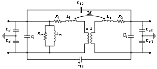Figure 1. Proposed model for transient state of transformer

The parameters of the model are defined as follows:

1. Ideal transformer with turns ratio n to consider the voltages ratio,

2. Rm and Lm: Core loss resistance and magnetization inductance to consider the no load current containing the core loss and magnetization current,

3. R1 and R2: The primary and secondary winding resistances including conductors skin effects,

4. C1 and C2: Series capacitances of the primary and secondary windings,

5. C12: Parallel capacitance between two windings,

6. Cg1 and Cg2: Capacitances between each winding and earth,

7. L1 and L2: Self inductances of windings, and

8. M: Mutual inductance between two windings.

The calculation of parameters with some proper experiments and using GA, which is an essential step in this model, is discussed in the next sections.

3. Tests and Measurements

For estimating transformer parameters and also checking the validity of this method, a three-phase transformer with power rating of 2.5 MVA is chosen as test object. This transformer consists of a disk-type high-voltage winding with 22 disks, 12 turns in each disk, and a layer-type low- voltage winding with four layers, 36 turns in each layer.

In present investigation all measurements were executed in the time domain to determine different TFs defined by the terminal conditions of the transformer which is illustrated in[16]. In the time domain, test objects are excited by low or high impulse voltages. The input and output transients are measured and analysed.

In low voltage measurements the amplitudes are usually 100 V to 2000 V. The shape of the impulse voltage depends on the test device and the test set-up. The bandwidth of the exciting signal should be as high as possible. Typical parameters of the impulse shapes are front times of 100 to 500 ns and time to half values of 40 to 200 μs. The spectral distribution of the time domain signals are calculated using Fast Fourier Transform (FFT). The quotient of output to input signal represents the TF in the frequency domain.

In figure 2 the necessary circuits for measuring frequency features in different conditions of terminal connections are shown. If the circuit of figure 2 is done in proposed model, disregarding the magnetic circuit of equivalent circuits, we will reach to figure 3. Notice that using coupling properties (figure 3(e)), M is considered in L_1p.

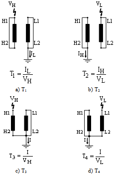Figure 2. Measuring circuits in various conditions of terminal connections

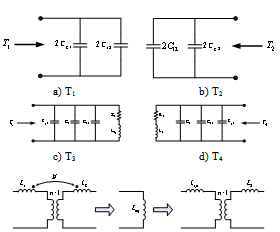Figure 3. The obtained equivalent circuits from running TFs to circuit of figure 1

4. Estimating the Model Parameters Using Genetic Algorithm

4.1. Genetic Algorithm

Genetic algorithm is a method which can be used for solving nonlinear equations and complex optimizing problems. GA is based on natural selection, providing solutions by generating a set of chromosomes referred to as a generation and repeatedly modifies a population of initial solutions. In contrast to more traditional numerical techniques, the parallel nature of the stochastic search done by GA often makes it very effective to arrive at global optimum. In GA approach, each design variable represented as a binary string (chromosome) of fixed length is evaluated by using a fitness function. If the search has to continue, the GA creates a new generation from the old one until a decision is made on the convergence. A crossover operator exchanges information contained in two parent individuals to produce two offspring and then replace the parents. The number of times the crossover operator is applied to the population is determined by the probability of crossover and the population size. A mutation operator randomly selects an individual from the population and then chooses two elements in this individual to exchange positions. A binary tournament selection strategy is used to select the fittest individuals where two individuals are selected at random from the population, and the better one is duplicated in the next generation. This cycle is repeated until an optimization criterion is reached[17].

GA generally includes the following sections:

Ø Gene: We call each independent variable "gene"; which is used directly or coded quantity of independent variable.

Ø Chromosome: A set or array of coded genes which is in a form of a response to optimizing problem.

Ø Population: The first population includes a specific number of chromosomes. These chromosomes are chosen from the whole searching space or randomly. Next generations of population in each level of genetic algorithm repetition are created by running genetic operators.

Ø The fitness function of chromosome: This is necessary in solving optimizing problem to define the optimization factor. The optimization factor of fitness function can be a goal function or can have relation with goal function. Fitness function is a device for evaluating each chromosome. It attributes each chromosome a number, which is specific to qualification of that chromosome.

4.2. GA Operators

The most important GA operators in MATLAB toolbox is defined as follows[18]:

Ø Reproduction: The reproduction operator reproduces each chromosome according to its standard function. So the chromosome which has better standard function will reproduce well in next generation.

Ø Crossover: The crossover operates on two chromosomes and reproduces two new chromosomes with a combination of their characteristics. For this chromosome obtained from reproduction are chosen for crossover by probability of P_c and another random number chooses the affection point of operator in chosen chromosomes. Crossover can be formed in several affection points, which is called multiple crossovers.

Ø Mutation: Mutation operator causes random changes in different individuals. For this, different individuals of population with probability of P_m are chosen. Then, a random number of affection point or mutation in chromosome will be determined and the bit will be completed. This operator also can run as multiple and in several points of chromosome will cause complement of bits.

4.3. GA Implementation

If Z_si is the simulated models response to the input X_ei and Z_xi the output vector got from experimental results, the goal of parameters identification is in this way: Z_si= Z_xi

According to the noise, numeral errors in simulation and the errors of measurement devices, there is never equality. So the best estimation for parameters is the estimation which decreases the sum of squares of errors for n couple of Y_si and Y_ei or in other words, increases the standard function to maximum:

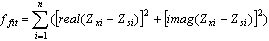(1)

Parameter identification is converted to an optimizing problem and can be solved using GA.

● The parameters which are used

For estimating parameters, the GA is done by two groups of different parameters. In the first level, we use T₁ and T₂ for estimating C_g1, C_g2 and C₁₂. So the parameters vector is like this: P₁=[C_g1 C_g2 C₁₂]

In the second level, for estimating of C₁, R₁ and L₁, we use the T₃; in this case, the parameters vector is like this: P₂=[C_eq1 L₁ R₁]

In the above relation, C_eq1 is the sum of C_g1, C₁₂ and C₁. The amount of C₁ can be obtained by C_g1 and C₁₂.

In the third level, we act like level two and use T₄ for estimating following parameters: P₃=[C_eq2 L₂ R₁]

C_eq2 is the sum of C_g2, C₁₂ and C₂.

● Runs the program

According to the facilities of MATLAB 7.5[18] and the toolbox of GA, for running the original program and estimating model parameters, this new facility is used. For using this toolbox at first we should enter "mfile". As the output, we can require various waveforms. Other quantities are given as default, but there are some changes in this quality; we will explain them bellow:

1. According to this fact that in checking of transient states, the amounts of resistances (in ohm), inductances (in mH) and capacitors (microfarad) are measured, it is better for increasing the speed of convergence in GA, to determine the first amount of variables personally.

2. At first, the probability of mutation is chosen high and at last, is selected low (because we close to the response). For this at first we use the uniform probability function with rate 0.5 and then, use the Gaussian probability function rates of 0.1 to 0.0001 by closing to the response at the problem.

3. The limiting amounts of running toolbox are assumed high amounts so that the end of running the program becomes an option for the user. The remaining settings of toolbox can be defined according to the type of the problem.

5. GA Execution and the Results

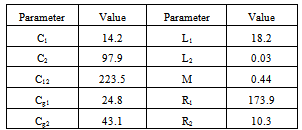
The obtained parameters of the model using GA method are listed in Table 1. For verifying the accuracy and validity of proposed method, we substitute the parameters obtained from TFs and get its frequency response by simulation. Thereafter, the results are compared.

Table 1. The amounts of estimated parameters using genetic algorithm (resistance (ohm), inductance (mH), capacitances (pF))

In figure 4 the results in frequencies of 10-200 kHz are compared. According to this figure we can say the accuracy of this model in definition of each four TFs is approximately the same. There are some differences between the results and simulation shows the acceptable accuracy of this model and also this method for estimating the parameters.

The deviations between the measurement and the calculation in figure 4 can be explained by:

² Using lumped elements for the presentation of distributed electric and magnetic field behaviour,

² Cable damping, transient characteristic of measuring devices, etc. can result in some effects, which are not considered in the model, and

² Manufacturing tolerances and parameter dispersions of the real winding arrangement.

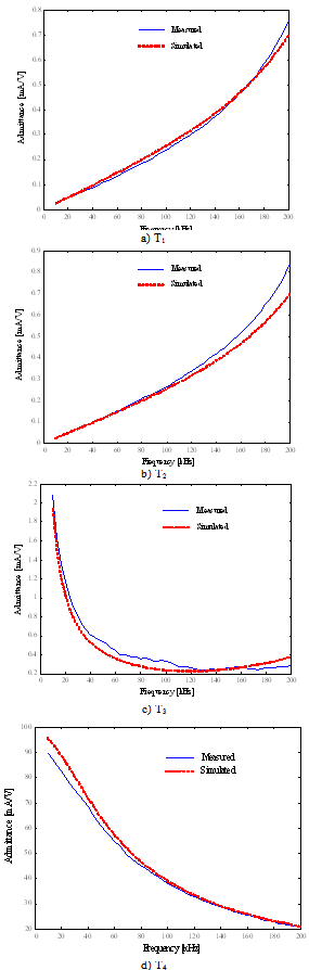Figure 4. Comparison of experimental an modeling results

6. Study of Some Physical Faults

As mentioned above, one of the most important applications of the proposed model is fault analysis and detection. Using a proper model the study of the fault effects on model parameters or terminal behaviour of transformer becomes straightforward. This section of paper gives an outlook about the fault detection of transformers using model.

6.1. Most Important Physical Faults

Two most important problems which always occur in fault investigation using the model are as follows:

An internal fault usually affects several parameters of the model[16]. This makes the fault analysis difficult.

The number of faults occurring in the transformer simultaneously is not generally clear, i.e. more than one type of fault might occur, so fault detections becomes more complicated.

Despite these problems, this paper can play an important role in transformer fault diagnosis. Some of the most important physical faults, which are given by authors, are listed below:

Turn to turn short circuit: This fault is generally caused due to insulation breakdown between the turns. By one turn to turn short circuit in high voltage winding (or in low voltage winding), the parameters n, R₁, L₁, and C₁ (or n, R₂, L₂ and C₂) will change more than other parameters[15]. The value of changes depends on the number of shortened turns.

Phase to ground fault: This fault is almost like the previously mentioned fault and network protection engineers are more interested in it[15]. Such fault modifies the C_g1, R₁, L₁ and C₁ (or C_g2, R₂, L₂ and C₂) more than other parameters, if occurs in high voltage side (or in low voltage side).

Axial displacement of winding: Due to extremely high forces resulting from system short circuit currents or other causes, the windings of transformer can be displaced axially [16]. A high-voltage or low-voltage winding axial displacement affects C₁₂ and M significantly.

Radial deformation of winding: This fault is very similar to axial displacement and considerably causes the variations of C₁₂, M, L₁ (or L₂) and C_g1 (or C_g2)[16].

Winding compaction: This fault occurs because of undesired forces and changes the height of winding[16]. Thus, the values of L₁ and C₁ (or L₂ and C₂) will vary significantly.

6.2. Effects of Model Parameters Variations on Terminal TFs

In order to achieve a sufficient database in fault analysis, the parameters of proposed model are changed separately to study their effects on terminal TFs. The results of the study are given in Table 2. Three types of changes are given in this Table, strong, weak and negligible. In the case of negligible changes, approximately no changes have been observed.

6.3. Discussion

As it is obvious in Table 2, some of parameters are more sensitive to a number of physical faults. Consequently, the proposed method can be used as a proper method for analysing the physical faults in transformers. Although, it should be noted that employing the given method in different transformers will reveal more knowledge for fault detection. Therefore, still more researches is required in this field.

Table 2. The effects of parameters variations on TFs (N: Negligible, W: Weak, S: Strong)

7. Conclusions

An appropriated model for analysing the transient state of transformer is proposed in this paper. The proposed model has following considerable features:

1. The time for its simulation in Electromagnetic Transients Program (EMTP) is low,

2. The model can be used with other models of network,

3. The model is simple, but accuracy in frequencies range of 10-200 kHz is acceptable,

4. The model parameters are obtained from GA; so there is no need to complex mathematical calculations for estimation of model parameters.

5. Considering the effects of faults on model is possible.

With the help of a three-phase 2.5 MVA and 6300/420 V transformer consisting of a disk high-voltage winding and a layer low-voltage winding it is shown that the model has a sufficient accuracy. The efficiency of proposed model in fault detection, as an important application of model, is shown in the last part of the paper.