Urban Rudez , Rafael Mihalic
University of Ljubljana, Faculty of electrical engineering, Trzaska 25, 1000 Ljubljana, Slovenia
Correspondence to: Urban Rudez , University of Ljubljana, Faculty of electrical engineering, Trzaska 25, 1000 Ljubljana, Slovenia.
| Email: |  |
Copyright © 2012 Scientific & Academic Publishing. All Rights Reserved.
Abstract
In recent decades, the advantages of a fast development in the computer and communication technology have been successfully harvested in the majority of technological areas for updating various mechanisms and processes. Power system control and protection is no exception. However, actual implementation of modern technologies into power system control and protection mechanisms depends on a country – in some of them it is rather dare and open-minded, in some of them it is very conventional. This also goes for underfrequency load shedding protection. In case of a sudden underfrequency conditions appearance in the power system only a centralized gathering of measurements and global actions (e.g. use of so-called WAMPAC technology – Wide Area Measurement Protection And Control) can represent an appropriate approach to a global problem. In such circumstances, underfrequency load shedding is often the last resort tool for avoiding a total power system blackout. It’s appropriate actions are of great importance both from technological and economical point of view. In this paper several different adaptive approaches are presented and compared in their efficiency via testing on two different dynamic power system models. First scheme is a typical adaptive scheme with calculation of active power deficit and equal distribution of the calculated value among four different load shedding steps. Second scheme involves some modification of shedding steps amount according to frequency first time derivative change between two steps. Other two schemes are of predictive type and shed load according to the prediction of minimal frequency value after active power deficit occurrence. Tests have shown that predictive schemes yield best results and therefore should be strongly considered as an actual possibility for power system implementation in the future.
Keywords:
Adaptive Control, Frequency Response, Power System Islanding, Power System Protection, Underfrequency Load Shedding
1. Introduction
Use of different protection mechanisms can ensure a safe operation of electric power system (EPS) by preventing operation in a so-called unwanted operating state. One of such circumstances is underfrequency operation. In Europe EPS operates synchronously at the nominal frequency value of 50 Hz. Every imbalance between generated and consumed active power reflects in the frequency deviation. When smaller amount of imbalance is in question, primary frequency control should be able to compensate this imbalance without any serious system consequences[1]. However, in case of higher amounts of imbalance, frequency control alone is not enough to cope with the disturbance within reasonable time scope. Consequently, frequency deviation reaches such values that an appropriate power system protection should be activated in order to prevent further problems. In case the frequency deviation is negative (i.e. frequency drop is caused by an excess of active power load compared to generation) corresponding power system protection is called underfrequency load shedding (UFLS).EPS operation at lowered frequency is especiallymercial turbine can withstand only a finite number of disturbances, which cause operation at rotating speed below 47.5 Hz. Here we should keep in mind that the time duration of such operation plays an important role at determining the number of allowed excursions below 47.5 Hz[2]. Therefore, in order to protect very expensive generating equipment, the operating limitations are said to be between 47.5 Hz and 52.5 Hz in Europe[1]. In case EPS frequency drops below 47.5 Hz, an undefrequency protection of generating units is activated that disconnects generating units from the grid. Consequently, frequency decays even faster and total EPS blackout can no longer be avoided. This reflects in major technical and financial problems and can without any doubt be considered as a critical state in a certain country[3]. In addition, building up a normal EPS operation takes a lot of time. Consequently, it is very reasonable to assure a high efficiency and reliability of UFLS protection.A concept of UFLS itself is rather simple: disconnecting such amount of load that the frequency does not drop below lowest acceptable limit as well as restore system frequency to acceptable limit (close to system nominal frequency) [4]. It is very useful to keep in mind the list of target performance features of an ideal UFLS scheme:- it should be simple due to its importance,- it should react fast. Consequently, as a human reaction time is not sufficiently small, automation is required,- it should be highly reliable. This feature prefers applications without global communication. However, the use of a global communication channels is necessary, as underfrequency operation is a global rather than a local issue[5],- it should be highly effective. Effectiveness is also closely related to automation whereas unnecessary measures have to be avoided,- it should disconnect as less load as possible.It is clear from the above list that it is impossible to fulfil all listed requirements in practice. However, by applying some compromises it is possible to sufficiently approach to the so-called target performance of UFLS protection. There are many different approaches available in the literature dealing with this matter. All of them have one thing in common: frequency is the only indicator of circumstances that require load shedding. A main reason for local frequency measurements not being a sole satisfactory input in UFLS methodology is the dynamic performance of the EPS at a sudden active power deficit occurrence[6]. Namely, frequency is a global system parameter only during the steady state, which in reality does not happen very often.In this paper first a concept of four different adaptive UFLS schemes, available in the literature is presented. Next, two used dynamic test system models are briefly presented in Section 3. Results of applying different adaptive UFLS schemes to two dynamic test system models are presented in Section 4. Finally, the conclusions are drawn in Section 5.
2. Adaptive UFLS Schemes
It is reasonable to expect that in the (near) future traditional UFLS schemes will be replaced by technically more sophisticated kind of schemes, called adaptive UFLS schemes. This name has been used throughout the literature as it describes their most typical feature: being able to adapt its reaction to the seriousness of the occurred disturbance.
2.1. Local Frequency versus COI Frequency
Due to already written fact that the frequency is in general a local rather than a global system parameter, for constructing an adaptive scheme a calculation of a Centre Of Inertia (COI) frequency is required. Namely, this is the only way for obtaining relevant information regarding a global state of a power system under question[5]. COI frequency can be calculated according to the following expression[6]: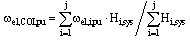 | (1) |
where ωel,COI,pu represents the electrical COI frequency in per unit, j is the number of all synchronous generators in the system, ωel,i,pu the electrical frequency of the i-th synchronous generator and Hi,sys the inertia constant of the i-th synchronous generator based on a common system base. COI inertia constant can be calculated as follows: | (2) |
where it is important to be aware of the difference between the synchronous generator inertia constant Hi and Hi,sys. The base for calculating Hi is the apparent nominal power of the i-th generation unit Sn,i. This is very convenient, as the typical value of Hi is in the range of 1-5 seconds[7]. However, when observing the multi generator system, the base should be some other value, typical for the whole system in question and not just for one of the generators. If we define a new system base Sbase,sys, inertia constants of all generators should be modified to the new base: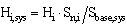 | (3) |
The COI frequency can therefore be calculated according to (1) – (3) in the system dispatch centre. The information regarding the calculated COI frequency has to be simultaneously communicated to the underfrequency relays, scattered across the system. This communication processes can be handled by using WAMS (Wide Area Measurement System), which enables transfer of these signals within reasonable and acceptable time frame.
2.2. Adaptive UFLS Scheme No. 1
The majority of adaptive UFLS schemes are based on calculation of an active power deficit Pdeficit that actually disturbed the observed power system[8]. According to the theory summarized in[6], this is possible by measuring the initial (at time t = 0) COI frequency first time derivative (FFTD) and by applying the multi-machine swing equation: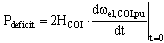 | (4) |
There are a few obstacles when using such a calculation[9]. However, they will not be discussed in this paper. Nevertheless, despite these problems many authors are still developing such schemes. A useful outcome of this doing is the growing level of implementation of newest microcontroller based relays in the actual power system, which can be considered as a base for applying adaptive power system protection.In this paper, we will consider a typical adaptive UFLS scheme that sheds equal portions of calculated Pdeficit in four frequency thresholds. This means that when each of four frequency thresholds is reached, Pdeficit/4 of load is disconnected. Selected frequency thresholds are 0.4 Hz apart (49.0 Hz, 48.6 Hz, 48.2 Hz and 47.8 Hz).
2.3. Adaptive UFLS Scheme No. 2
In previous subsection a most common approach to adaptive UFLS is described. However, many authors suggest different modifications of such approach. One of such suggestions is described in[5] where it has been shown that by monitoring COI FFTD, very valuable information regarding the activity of a frequency control can be obtained. Graphically this is summarized in Figure 1.A sum of Δ1, Δ2 and Δ3 equals to a total contribution of a frequency control between load shedding step 1 and load shedding step 3 in the process of regaining the balance between the generation and a consumption of active power in the system. It should be noted that by obtaining this information, the total amount of disconnected load can be reduced accordingly. Namely, this is one of advantages of such modification: fewer loads are disconnected compared to adaptive schemes without this modification, where the system still remains safe from a blackout.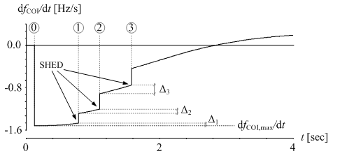 | Figure 1. Monitoring the activity of frequency control by measuring FFTD |
2.4. Adaptive UFLS Scheme No. 3
In[10] an introduction to a new sub-type of adaptive UFLS schemes, the so-called “predictive UFLS schemes”, can be found. Their operation is based on predicting the power system frequency response in advance. Many different possibilities exist how to achieve that. However, in this section, a methodology presented in[10] is considered.The methodology is based on predicting the COI frequency second time derivative (FSTD). Namely, FSTD can be considered as an acceleration of the frequency and therefore reflects the level of frequency control activity, as this has the most crucial influence on the actual frequency trajectory. In[10] it has been shown that FSTD, after a sudden active power deficit appears in the system, maintains some typical shape with respect to time, regardless of the amount of active power deficit or the parameters of different types of regulators. This shape can suitably be mathematically represented with an exponential function. An example of a dynamic simulation, applying such predictive UFLS scheme, is given in Figure 2. By continuous approximation of FSTD with an exponential curve (iterative procedure), it is possible to forecast minimal frequency, if no further actions are undertaken (i.e. load shedding). According to this value, load shedding is activated with fixed time delay (250 ms) between two subsequent steps as long as the forecasted value of the minimal frequency is said to drop below 47.5 Hz.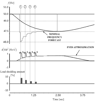 | Figure 2. An example of a dynamic simulation by applying predictive UFLS scheme |
2.5. Adaptive UFLS Scheme No. 4
In the very near future, authors will publish a paper, containing a detailed description of another predictive subtype of adaptive UFLS schemes. This methodology will be actually an upgrade of the one in Section 2.4, where the improvements are:- frequency first time derivative (FFTD) is used instead of FSTD,- prediction of future frequency trajectory (its minimal value) is calculated with a single algebraic equation instead of using iterative procedure.The main idea of this approach can be explained by analysing a locus diagram of a COI frequency versus FFTD after a sudden deficit of active power appears in the system. An example of such locus diagram is depicted in Figure 3a. In the steady state frequency is equal to nominal value of 50 Hz and FFTD equals zero. After a sudden deficit appears, frequency cannot change instantly. However, FFTD can change instantly from 0 to the maximal value (minimal to be exact as the FFTD is negative when the active power deficit appears). When the frequency actually starts to decay, primary frequency control is regaining balance between the production and the consumption of active power and consequently, FFTD is again approaching to a value of 0. At this point, the frequency is at its lowest value. After post-fault steady state is obtained, the power system frequency is less than nominal value due to a permanent droop characteristic of the turbine controllers in the system. If we take a look at the trajectory in this diagram (Figure 3a) it is clear that its shape can be described as a spiral.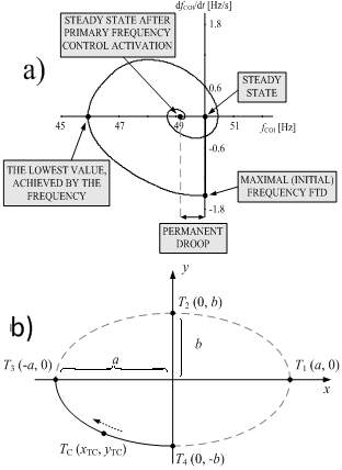 | Figure 3. a) Locus diagram of a COI frequency versus FFTD, b) general ellipse definition |
However, in order to predict the behaviour of the system only a part of a spiral is relevant. For a purpose of approximation a part of an ellipse can be used, which is depicted in Figure 3b with a thick black curve. A common equation of an ellipse can be written as follows: | (4) |
where a is called the major radius and b is the minor radius of the ellipse. a and b are one half of the major and minor diameters, respectively. By comparing Figure 3a and Figure 3b it is clear that we can consider fCOI for a and dfCOI/dt for b. Therefore, by measuring the frequency and FFTD it is possible to predict the lowest value achieved by the frequency (fMIN,forecast) with a simple algebraic calculation, derived from ellipse equation.
3. Dynamic Test System Models
3.1. IEEE 9 Bus Test System
For testing UFLS schemes efficiency, some authors (e.g. in[11]) use a dynamic model of an IEEE 9 bus test system (Figure 4). This model is described in details in[7] with all necessary parameters. The model consists of three synchronous generators together with corresponding block transformers, six transmission lines and three power system loads. In order to use this model for UFLS purposes, a slight modification had to be introduced: an infinite power source (GRID) was connected to bus 4 via switch S-GRID. In this way, many different power conditions can be simulated simply by changing the production of three generating units and the consumption of three power system loads. In addition, GRID in all cases supplies/consumes enough power to meet the power balance in a steady state. Simply by disconnecting S-GRID at a certain moment during simulation, a power system island is formed, with a certain imbalance between the production and a consumption of active and reactive power. In this paper, circumstances with a lack of active power were simulated, which causes a power system frequency to decay.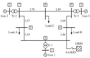 | Figure 4. The model of the IEEE 9 bus test system |
An example of a simulation of such islanding is given in Figure 5. The graph presents FFTD of all three synchronous generators with respect to time. It can be clearly seen that the generators react differently, according to the electrical distance from the fault (bus 4) and generator parameters (especially inertia constant).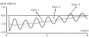 | Figure 5. An example of a different generators reaction to infinite power source disconnection |
3.2. A North-Western Part of a Slovenian Power System
In order to perform as realistic test as possible, a model of a real power system has to be included into analysis. Concerning this, we have used a dynamic model of a north-western part of a Slovenian power system, with a nominal voltage of 110 kV (Figure 6). This part of a system is suitable for islanding simulations due to a fact that there is only one substation (Divaca) connecting it to the rest of a Slovenian power system. Therefore, in case any problems occur in this substation, islanding operation cannot be avoided.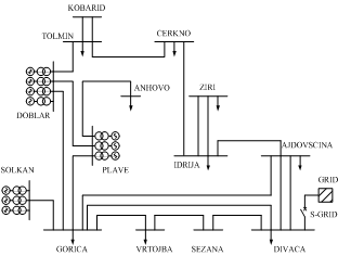 | Figure 6. The model of a north-western part of Slovenian power system |
This model consists of ten synchronous generators with corresponding block transformers, nine power system loads and twenty transmission lines. Similar than in Subsection 3.2 an infinite power source is added to the model, which is connected via switch S-GRID to substation Divaca. By disconnecting S-GRID, a transmission into the island operation is simulated.It should be noted that one important difference exist compared to IEEE 9 bus test system: presence of ohmic losses. Namely, ohmic losses should be treated as a part of a power system demand and following Figure 5, they have some additional effect on power system oscillations after disconnection of S-GRID. However, this issue has already been presented and analysed in[5].
4. UFLS Comparison Results
In this Section, first a dynamic frequency response for applying different adaptive UFLS schemes will be shown. As two test systems are considered in this paper, a frequency response will be shown for both. Due to several possible disturbances that might aggravate the system (different values of active power deficit), only one dynamic response with respect to time has been shown for each test system. However, taking into account a fact that the frequency drop below 47.5 Hz has been prevented in all simulated cases, a graphical representation of efficiency of different schemes has been used as in[5]. Therefore, in Section 4.2 two graphs are shown from which it can be clearly seen which of the schemes acquires best results for all kinds of active power deficit values.
4.1. Examples of a Dynamic Simulation
First, let us take a look at the circumstances of 220 MW active power deficit in the IEEE 9 bus test system. Figure 7 depicts a power system frequency with respect to time for applying all four presented adaptive UFLS schemes. It can be clearly seen from Figure 7 that the frequency drops lower when using scheme No. 2 compared to circumstances with scheme No. 1. The reason for this is a modification of all shedding steps, according to frequency control activation. This can especially be seen at frequency threshold 48.2 Hz, where load disconnection is completely avoided in case of scheme No. 2. In this way, fewer loads are disconnected on the account of increasing active power production. However, even though the frequency drop is consequently lower, the lowest acceptable limit of 47.5 Hz has not been violated.If we observe the frequency response of adaptive UFLS scheme No. 3, a first thing that is obvious is that frequency just barely reaches 47.5 Hz. This is due to the fact that this scheme is parameterized in such a way, that load shedding is initiated whenever lowest frequency forecast drops below 47.5 Hz. This also goes for UFLS scheme No. 4. Re- parameterization can be made easily for both schemes (No. 3 and No. 4) in order to increase this limit. However, by using the value of 47.5 H, the results of the scheme are brought to its limits, as manoeuvre space available for load shedding can be considered a frequency band between 49.0 Hz (when the load shedding should be initiated) and 47.5 Hz (the limit for underfrequency protection of production units). As clearly in all four cases frequency drop below 47.5 Hz is successfully prevented, the next criteria for evaluation of the scheme’s efficiency can be the total amount of disconnected load. When using the adaptive UFLS scheme No. 1, 53.2 % of the total system load is disconnected, in case of using scheme No. 2, 39.7 % of total load is disconnected, in case of using scheme No. 3, 29.5 % of load is disconnected and in case of using scheme No. 4 29.9 % of load is disconnected. Considering scheme No. 1 results as a reference, by using scheme No. 2 a little more than 25 % less load is disconnected. However, by using schemes No. 3 and No. 4 even 44 % more loads remains supplied (schemes No. 3 and No. 4 have very similar results). Especially the results of the latter two schemes can be treated as a remarkable improvement.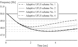 | Figure 7. Frequency response of an IEEE 9 bus test system, suffering 220 MW deficit applying different adaptive UFLS schemes |
Next, let us take a look at the results of similar analysis by applying all four adaptive UFLS schemes in the dynamic model of a north-western part of the Slovenian power system, suffering 75 MW of active power deficit (Figure 8). It can clearly be seen that the initial FFTD is higher (frequency drop is more severe) than in Figure 7. However, modifications of load shedding steps, made by scheme No. 2, have similar effect that in Figure 7. Most obvious consequence of this modification is leaving out the load shedding step at frequency threshold 47.8 Hz, which in case of scheme No. 1 causes over-shedding and also frequency overshoot (frequency increase above nominal value, despite the fact that the initial problem was underfrequency). Again, by using schemes No. 3 and No. 4 frequency drop is once again lower, but the “survival” of the power system island is not jeopardized as this is a consequence of intentional parameterization of both schemes.In this analysis frequency drop below 47.5 Hz is also successfully prevented. Therefore, it is reasonable to observe the next criteria for evaluation of the scheme’s efficiency: the total amount of disconnected load. When using the adaptive UFLS scheme No. 1, 63.4 % of the total system load is disconnected, in case of using scheme No. 2, 54.0 % of total load is disconnected and in case of using scheme No. 3, 46.2 % of load is disconnected. Again, scheme No. 4 yields similar results than scheme No. 3, which means that 49.8 % of load is disconnected. Considering scheme No. 1 as a reference, by using scheme No. 2 almost 15 % less load is disconnected and by using scheme No. 3 even more than 27 % more load remains supplied. Scheme No. 4 has slightly worse results than scheme No. 3 as more than 21 % of load is prevented from tripping. Even though all the percent improvements are lower than in the case of IEEE 9 bus test system, this can still be treated as a remarkable improvement. Especially taking into account the fact that the FFTD value was higher and consequently frequency conditions were more severe in all simulations.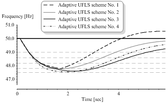 | Figure 8. Frequency response of a north-western part of Slovenian power system, suffering 75 MW deficit applying different adaptive UFLS schemes |
4.2. Summary of Results
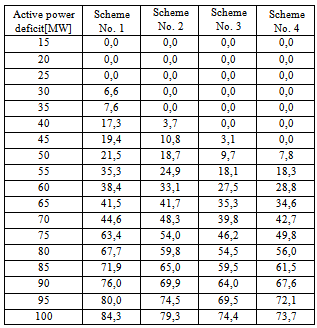
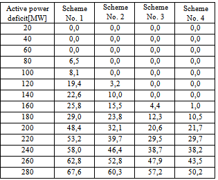
It is very important to test UFLS scheme operation in all possible conditions that might appear in a power system. However, showing the results of all individual dynamic simulations is not appropriate for papers with limitations in length. Therefore, authors used similar representation of results as in[5] (Figure 9 for IEEE 9 bus test system and Figure 10 for a model of north-western part of Slovenian power system). On the horizontal axis the simulated values of active power deficit are given and on the vertical axis the total load shedding amount for each individual simulated case. It should be noted that for each simulation the prevention of frequency drop below 47.5 Hz has been achieved, even though this cannot be seen from Figure 9 and Figure 10. In Tables 1 and 2, numerical results of the same simulations are given.Table 1. Numerical representation of results performed on IEEE 9 bus test system model
 |
| |
|
Table 2. Numerical representation of results performed on a model of north-western part of Slovenian power system
 |
| |
|
First let us take a look at the results of IEEE 9 bus test system (Figure 9). Adaptive UFLS schemes No. 3 and No. 4 yields by far best results. In the circumstances of lower deficit values (less that 160 MW) none of the loads are disconnected and therefore, frequency control alone regains the active power balance in the system. Higher deficit value is simulated, more severe circumstances appear and more difficult it is to obtain significant improvement compared to scheme No. 1. Nevertheless, adaptive schemes No. 3 and No. 4 show the most promising results compared to other two tested schemes. Among those two schemes, authors would like to emphasize the fact that operation of scheme No. 4 is much more simple and robust than of scheme No. 3 despite very similar results. In addition, the total load shedding amount is almost linearly dependent on simulated value of the deficit when using schemes No. 2, No. 3 and No. 4. This is not the case with scheme No. 1, as a result of only its first part (active power deficit calculation by using (4)) being actually adaptive. On the other hand schemes No. 2, No. 3 and No. 4 are showing its adaptive character from the time load shedding begins until the FFTD reaches value of zero.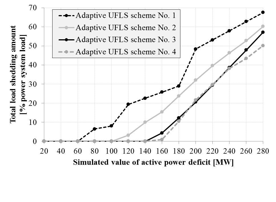 | Figure 9. Summary of results performed on IEEE 9 bus test system model |
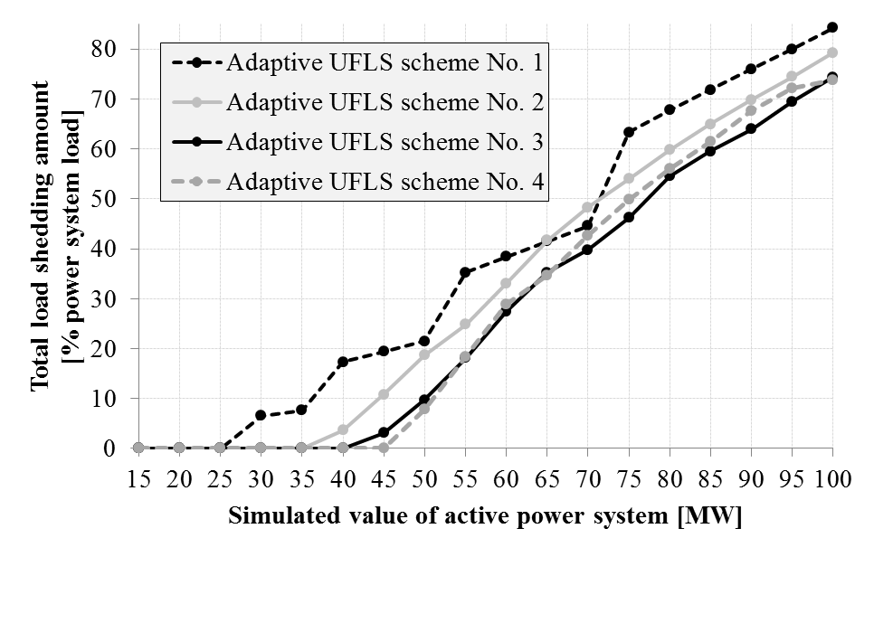 | Figure 10. Summary of results performed on a model of north-western part of Slovenian power system |
Let us now take a look at the results of the second test system (Figure 10). As higher values of FFTD are a consequence of lower values of system inertia HCOI, the improvements compared to the results of scheme No. 1 are less significant. It even happens that at Pdef = 70 MW scheme No. 2 sheds more load than scheme No. 1, despite its adaptive modifications during frequency fall. Nevertheless, overall performance of scheme No. 2 is still much better that of scheme No. 1. Similar than in Figure 9 schemes No. 3 and No. 4 yield best results and shed no load for deficits lower that 45 MW and 50 MW, respectively.
5. Conclusions
According to the low effectiveness of traditional UFLS schemes it would be reasonable to upgrade the current status of UFLS protection, especially when considering an enormous advance in communication and computer technology during the last few decades. However, a special attention should be given to a process of choosing among many available UFLS methodologies. Main focus of the paper was to clearly show, which adaptive types of UFLS schemes are to be considered in the future for actual implementation. It has previously been indicated that typical adaptive UFLS schemes (with calculating the actual active power deficit in the system) do not meet the practical requirements that are necessary for the actual implementation in the power system. On the other hand, predictive sub-type of adaptive UFLS schemes is more appropriate for actual implementation. Of course, as system conditions in question are a global rather than a local issue, a certain level of communication is required in order to calculate the COI frequency in the dispatch center and to forward the information regarding necessary action to geographically scattered underfrequency relays. One must be aware that this kind of communication is an unavoidable part of all adaptive UFLS schemes. Nevertheless, predictive schemes acquire enough information regarding the system reaction to a disturbance simply by observing either the FSTD or FFTD and disconnect load accordingly. In this way, very good results are obtained which far exceed the results of other tested adaptive UFLS schemes.Four adaptive UFLS schemes have been tested for various system conditions (i.e. active power imbalances) on two test system models. First scheme has been proven in[9] to be very sensitive to load variations due to voltage changes. Considering these modifications in active power deficit calculation causes the scheme to be very much dependent on a lot of on-line power system data and therefore, authors find it unsuitable for actual implementation in a power system. Even though second scheme is a modification of the first one, it still suffers from the same problem. However, it introduces some valuable solutions for monitoring the power system response to a disturbance. The third scheme is according to our knowledge a pioneer in predictive subtype of UFLS schemes. It discovers a new possibility of predicting the system frequency in advance and sheds load accordingly. However, frequency second time derivative is used to obtain the prediction in an iterative manner and this might also not be accepted in practice. Nevertheless, fourth scheme takes another step further and avoids two biggest drawbacks of the third scheme, while still maintains its quality performance.Keeping above discussion aside, it has been shown that both predictive subtypes of UFLS schemes yield best results in all simulated cases. For evaluation of the results the criteria of lowest amount of disconnected load has been chosen, while it has been verified that the system frequency remains above the critical limit of 47.5 Hz at all times.Therefore, according to our analysis authors suggest that more attention should be given to predictive schemes in the future, especially to scheme 4, which is based on rather straightforward and transparent relation between system frequency and its first time derivative. Namely, it has to be stressed that usually most simple concepts usually represent the best solution.
ACKNOWLEDGEMENTS
This work was supported by a Slovenian Research Agency as a part of the research program Electric Power Systems, P2-356.
References
| [1] | UCTE, "Load – frequency control and performance, Appendix 1". Final version, 20.07.2004. |
| [2] | An American National Standard, "IEEE guide for abnormal frequency protection for power generating plants", ANSI/IEEE C37.106-1987 (Reaffirmed 1992). |
| [3] | University of Ljubljana, Faculty of electrical engineering, "Slovenian power system operation during natural and other disasters", Final report, April 2008. |
| [4] | IEEE Power Engineering Society, "IEEE Guide for the Application of Protective Relays Used for Abnormal Frequency Load Shedding and Restoration", IEEE Std C37.117TM-2007, 24 August 2007. |
| [5] | U. Rudez, R. Mihalic, "Monitoring the First Frequency Derivative to Improve Adaptive Underfrequency Load-Shedding Schemes", IEEE, Transactions On Power Systems, vol. 26, No. 2, pp. 839 – 846, 2011. |
| [6] | U. Rudež, R. Mihalic, "The theory behind using the first frequency derivate for underfrequency load shedding purposes", 19. Internationl expert meeting Power engineering, 11. - 13. May 2010, Maribor, Slovenia. |
| [7] | P. M. Anderson, A. A. Fouad, "Power System Control and Stability", The Iowa State University Press, First Edition, 1977. |
| [8] | P.M. Anderson, M. Mirheydar, "A Low Order System Frequency Response Model, " IEEE, Transactions On Power Systems, vol. 5, No. 3, pp. 720-729, August 1990. |
| [9] | U. Rudez, R. Mihalic, "Analysis of Underfrequency Load Shedding Using a Frequency Gradient", IEEE, Transactions On Power Delivery, vol. 26, No. 2, pp. 565 - 575, 2011. |
| [10] | U. Rudez, R. Mihalic, "A novel approach to underfrequency load shedding", Electric Power System Research, vol. 81, Issue 2, pp. 636–643, February 2011. |
| [11] | V. V. Terzija, "Adaptive underfrequency load shedding based on the magnitude of the disturbance estimation, " IEEE, Transactions On Power Systems, vol. 21, Issue 3, pp. 1260-1266, August 2006. |
 Abstract
 Reference
 Full-Text PDF
 Full-Text HTML