1. Introduction

In recent years, with the opening of electricity market, electrical power systems load forecasting play an important role for electrical power operation. Accurate load forecast will lead to appropriate operation and planning for the power system, thus achieving a lower operating cost and higher reliability of electricity supply. Short-term load forecasting (STLF) of electric power not only plays a very important role in operation scheduling, like economic emission dispatch, unit commitment, energy transactions, and fuel purchasing, but also has a significant impact on the secure operation of power system[1, 2]. Short-term load forecasting aims to predict electric loads for a period of minutes, hours, days or weeks. The quality of the short-term load forecasts with lead time ranging from one hour to several days ahead has a significant impact on the efficiency of operation of any power utility[3– 5]. The objectives of the STLF are[6]:

● To derive the scheduling function that determines the most economic load dispatch with operational constraints and policies, environmental and equipment limitations.

● To insure the security of the power system at any time point.

● To provide system dispatchers with timely information.

The time series model extrapolates historical load data to predict the future loads. It assumes a stationary load series and retains normal distribution characteristics. When the historical load data does not represent the conditions, the accuracy of the forecast by the time series model decreases[7]. The main principle behind the linear regression method is to use the common relationships among all variables in the model to predict the relative change of one variable by the changes in other variables. Owing to the importance of STLF, research in this area in the last years has resulted in the development of numerous forecasting methods[8]. These methods are mainly classified into two categories: classical approaches and artificial intelligence (AI) based techniques. Classical approaches are based on various statistical modeling methods. These approaches forecast future values of the load by using a mathematical combination of previous values of the load and other variable such as weather data. Classical STLF approaches use regression exponential smoothing, Box-Jenkins, autoregressive integrated moving average (ARIMA) models and Kalman filters. Recently several research groups have studied the use of artificial neural networks (ANNs) models and Fuzzy neural networks (FNNs) models for load forecasting[9]. With the development of AI in recent years, people become able to forecast using FNN and ANN with the back propagation method. Although the back propagation method has solved a number of practical problems, its poor convergence and speed can somewhat deter engineers. Meanwhile, a conventional ANN model sometimes can suffer from a sub-optimization problem[10, 11].

In this paper a new approach using Curve fitting prediction optimized by genetic algorithm is used for short – term load forecasting. This method combined with genetic algorithms is used for obtaining the optimum parameters of Gaussian model which used as the fitting function in the prediction methods. The prediction model depends on the process of training of the CFP program. The predicted values give a great agreement with available experimental data for short-term load. It is found that the proposed method can provide more accurate results than the conventional techniques.

2. Load Forecasting Modeling

The load series, y(t) is modelled as the output form a linear filter that has a random series input a(t), which is called a white noise as shown in Fig. (1). This random input has a zero mean unknown fixed variance . Depending on the characteristic of the linear filter, different models of STLF can be classified as follows [4, 5]:

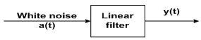Figure 1. Load time series modelling

2.1. Autoregressive Model AR(p)

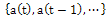
In this model, the current value of the time series process y(t) is expressed as a linear combination of its previous values 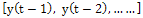and a random noise a(t). The order of this series depends on the oldest previous value at which y(t) is regressed on. An autoregressive process of order , AR(p), can be written as:

(1)

By introducing the backshift operator the defines , and consequently 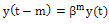, Equation (1) can be expressed as:

(2)

where,

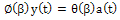
2.2. Moving Average Model MA(q)

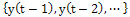
In this model, the current value of the time series y(t) is expressed linearly in terms of current and previous values of a white noise series . This noise series is constructed from the forecast errors or residuals when load observations become available. The order of this procedure depends on the oldest noise value at which y(t) is regressed on. A moving average of order q, MA(q), can be written as:

(3)

A similar application of the backshift operator on the white series will allow equation (3) to be expressed as:

(4)

where,

2.3. Autoregressive Moving Average Model ARMA(p,q)

In this model, the current value of the time series y(t) is expressed linearly in terms of its values of previous periods and in terms of current and previous values of a white noise 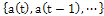. The order of the ARMA model is selected by both of the oldest previous value of the series and the oldest white noise value at which y(t) is regressed on. An ARMA of order p and q, ARMA(p, q), can be written as:

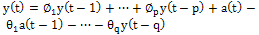(5)

By using the backshift operator, equation (5) can be expressed in the following form

(6)

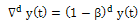
2.4. Autoregressive Integrated Moving Average Model ARIMA(p, d, q)

The time series defined previously as AR, MA or ARMA process is called a stationary process. This means that, the mean of the series of any of these processes and covariance among its observation does not change with time. If the process is non-stationary, transformation of the series to a stationary process has to be performed first. This can be achieved, for the time series that are non-stationary in the mean, by differencing process. By introducing the operator, a differenced time series of first order can be written as:

(7)

Consequently, an order d differenced time series can be expressed as:

(8)

The differenced stationary series can be modelled as an AR, MA or ARMA to yield an ARI, IMA or ARIMA time series processes. For a series that needs to be differenced times and has order p and q for the AR and MA components, ARIMA(p, d, q) can be expressed as:

(9)

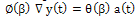
2.5. Seasonal Process of Load Modelling

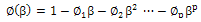
The load demand is a highly periodic process. The general ARIMA model should be altered to accommodate this periodicity (e.g., the load at 10 AM Tuesday is related to the load at 10 AM Monday). Therefore, the seasonal time series can be modelled as an AR, MA, ARMA or an ARIMA seasonal process similar to the non-seasonal time series. The general multivariate model (p, d, q)•(P, D, Q) for a time series model can be written in the form:

(10)

where,

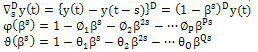where, s is equal to the number of samples per day (e.g., s =24 for hourly load , s =7 for daily load). The general class of models for periodic data with period 24 hours can be expressed as:

(11)

3. The Proposed Techniques

The proposed algorithm is based on Curve Fitting Prediction and genetic algorithms. The two techniques could be described as follows:

3.1. Curve Fitting Prediction

Curve Fitting Prediction software is a collection of graphical user interfaces (GUIs) and prediction functions for curve and surface fitting that operate in the MATLAB technical computing environment [1]. A typical flowchart for curve fitting prediction methods is shown in Fig (2).

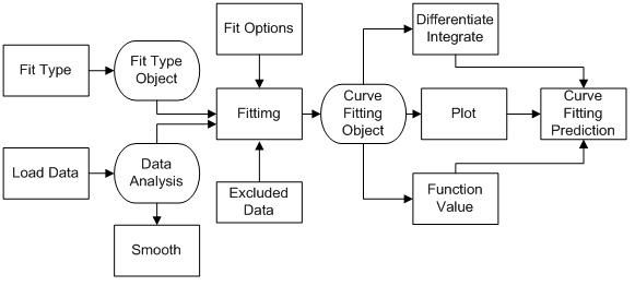Figure 2. A typical flowchart for curve fitting prediction methods

The toolbox supplements with [1]:

● Data pre-processing capabilities, such as sectioning, excluding data, and smoothing.

● Data fitting using parametric and nonparametric models:

● The toolbox includes a library of parametric models, with polynomials, exponentials, rationales, sums of Gaussians, Fourier polynomials, and many others.

● It can also define custom models to precisely reflect the goals of the data analysis.

● Nonparametric models are available through a variety of smoothers and interpolates.

● Fitting methods for linear least squares, nonlinear least squares, weighted least squares, constrained least squares, and robust fitting are available

● Data and fit statistics to assist in analysing the models

● Post processing capabilities that allow interpolating, extrapolating, differentiating, and integrating the fit.

The following statistics to determine the best fit [1]:

■ SSE is the sum of squares of errors of the fit. A value closer to zero indicates a fit that is more useful for prediction.

■ RMSE is the root mean squared error or standard error. A value closer to zero indicates a fit that is more useful for prediction.

Smoothing estimates the centre of the distribution of the response at each predictor. It invalidates the assumption that errors in the data are independent, and so also invalidates the methods used to compute confidence and prediction intervals. Accordingly, once a parametric model is identified through smoothing, the original data should be passed to the fit function.

3.2. Examining the Numerical Fit Results

There are two types of numerical fit results displayed in the Fitting GUI: goodness of fit statistics and confidence intervals on the fitted coefficients. The goodness of fit statistics helps to determine how well the curve fits the data. The confidence intervals on the coefficients determine their accuracy. The fitting function used in this paper is the Gaussian model function:

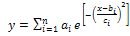(12)

where; a is the amplitude, b is the centred (location), c is related to the peak width, n is the number of peaks to fit, and , in this paper the value of n =5[1]. In this paper, the SSE and the RMSE are used to determine the best fit by using Genetic Algorithms.

3.3. Procedure of the proposed model

The steps of the procedure of the proposed model are:

■ The load data for the specific day is training using the first three week day data to the CFP using Gaussian function and RMSE method to get the curve fitting.

■ The values of a, b and c is improved using GAs to minimize the RMSE as possible.

■ After the improvement of the RMSE the CFP program used the fitting curve equation to predict and forecast the load of that day in the fourth week.

■ The prediction data compared with the actual one and evaluate the error value.

3.4. Genetic Algorithms

Genetic algorithms are biologically inspired techniques used for optimization. GAs was formally introduced by Johan Holland at university of Michigan, US, in 70s[1,13]. They are less prone to stick in local minima. In GAs a solution to the problem is given (as a chromosome). The GAs then creates populations of solution to apply genetic operators as crossover and mutation to evolve the new possible solution[1,13]. It finds the fitness function for possible solutions and finds the optimal one. Following is the Pseudo code of GAs. In crossover operator a crossover point is selected in parent chromosome. All data beyond that point in parent chromosome is swapped between the two parent chromosomes. The resulting chromosomes are called children. Crossover operation is graphically illustrated in Fig. (3).

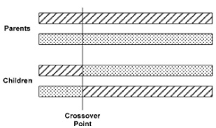Figure 3. Crossover Operator of GAs

In mutation operator GA changes randomly values of some genes of parents. The operation of mutation operator is shown in Fig. (4).

The elite child is those strings in which have the best fitness value and these are gone in next generation as it was. The used objective function is simply the accumulated squared error, which has the form [1]:

(13)

where, m is the number of input load data

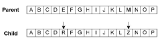Figure 4. Mutation operator of GAs

The problem is now reduced to the determination of the optimum values of parameters a, b and c from equation (12) subject to the satisfaction of the objective function given by equation (13), using GAs.

4. Practical Applications

The proposed method is used to find the accurate forecasting model of the hourly load through an application on Zagazig city – Egypt. The actual power load data taken from the Egyptian Electricity Authority of Canal Zone, Sharkia Network. Actual record data is used to perform the study. The data given represents the hourly load for the year 2007 [1].

5. Results

The proposed curve fitting prediction optimized by Genetic Algorithm to identify the model for STLF has been implemented on the practical load data. The historical load data shown in Table 1 were used to develop the proposed model, and the model was then used to forecast the testing load data.

Table 1. Load data used for load forecast Load type Historical load data Testing load data Winter Season 1 January – 23January 2007 24 January – 30 January 2007

Table 2. The (MPRE) mean percent relative error Weekday MPRE % Saturday -0.8 Sunday 0.15 Monday 0.2 Tuesday 0.11 Wednesday -0.6 Thursday -0.24 Friday -0.38

Fig. (5) depicts the optimization process of the best parameter values obtained by the curve fitting prediction and optimized by Genetic Algorithm. The hourly load forecasting results of the proposed method are depicted in Figs. (6 – 12), Fig. (13) shows the percentage error of the proposed method. Table 2 represents the mean percent relative error (MPRE) for the week days.

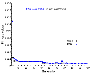Figure 5. Optimization of the best parameter values in the proposed method using GAs

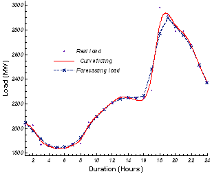
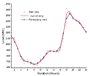Figure 6. Actual, curve fitting and Forecasting load results of proposed method in the case of Monday

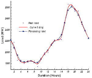
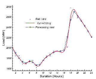Figure 7. Actual, curve fitting and Forecasting load results of proposed method in the case of Tuesday

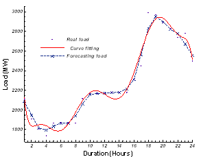
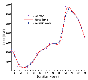Figure 8. Actual, curve fitting and Forecasting load results of proposed method in the case of Wednesday

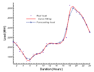
Figure 9. Actual, curve fitting and Forecasting load results of proposed method in the case of Thursday

Figure 10. Actual, curve fitting and Forecasting load results of proposed method in the case of Friday

Figure 11. Actual, curve fitting and Forecasting load results of proposed method in the case of Saturday

Figure 12. Actual, curve fitting and Forecasting load results of proposed method in the case of Sunday

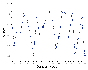Figure 13. The average percentage relative error

6. Conclusions

This paper introduces a new approach to improve the short – term load forecasting, which was a difficult task using conventional methods. The proposed approach uses curve fitting optimized by genetic algorithms. Load forecasting plays a dominant part in the economic optimization and secure operation of electrical power systems. The high cost and limited resources of primary energy inputs, together with the development of computer and control technologies, provide incentive for the further development of techniques for load prediction for the system operation. The objective of the research is to design a compact, fast and accurate model. So, the new approach of design was based on finding a method for minimizing the input variables and the training set in order to speed up the model. The forecasting model presented in this paper shows that the proper selection of input variables and training vectors results a very low training and forecasting time. The accuracy of the proposed model is excellent. It showed a mean percentage relative error (MPRE) less than 1%.