1. Introduction

Electromagnetic wave amplification by nonlinear wave mixing has been studied extensively in the context of nonlinear optics [1]. It has been well established that we can amplify a relatively low power input wave, by using another wave of high intensity, which is called the pump wave, in a nonlinear medium [2]. The theory of electromagnetic wave amplification via nonlinear wave mixing involves the transfer of energy from the pump wave to the input wave as a result of nonlinear coupling in a medium that exhibits a strong nonlinear response under excitation [3]. The nonlinear wave mixing theory has been mostly investigated experimentally rather than computationally, especially for wave amplification purposes. The most important reason behind this trend is that, this concept is almost always studied in the micrometer or nanometer wavelength range, and yet the required medium length to observe any significant nonlinear effect is in the milimeter or centimeter range, which requires an extremely high computational cost for obtaining meaningful results, particularly for the purpose of wave amplification.

Furthermore, based on the current concept of wave amplification via nonlinear wave mixing a.k.a parametric amplification, it is impossible to achieve a non-negligible wave amplification in a few micron sized gain medium or a cavity. The required gain medium length for significant parametric amplification is mostly on the order of centimeters [4]. For this reason, the concept of parametric amplification is not feasible to be used for optical microsystems. In this paper, we have carried out a computational analysis that aims to show that it is possible to amplify a low power stimulus wave by mixing it with an intense pump wave of very short duration, in a wide range of frequencies and with a very large gain coefficient, inside a low-loss micro-cavity of several micrometers of length, by maximizing the stored pump wave energy in the cavity.

We will first discuss about high energy storage in low-loss cavities. A low-loss cavity has a high quality factor, which is a measure of the energy storage capability of a cavity. Then, we will discuss about wave propagation in nonlinear dispersive media, and formulate our problem along with it’s finite difference time domain implementation. Finally, we will present our results through a set of simulations and we will try to depict that a very high gain optical parametric amplification is possible in a low-loss micro-cavity, when the correct pump wave frequencies that maximize the stored intracavity energy are chosen.

2. Intracavity Energy Density and the Cavity Quality (Q) Factor

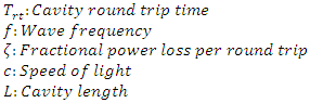
The Q factor is a measure of the energy storage capability of a cavity. A high Q value means that high energy can be stored in the cavity. It depends on the length of the cavity, the values of the reflection coefficients of the cavity walls, the frequency of the wave that is propagating inside the cavity, the total absorption coefficient of the medium between the cavity walls, and any kind of diffraction or scattering loss that can occur inside a cavity [14-16]. The Q factor of a cavity is defined as

(1)

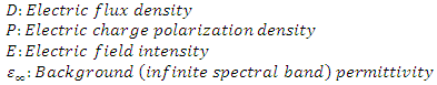
The stored electric energy density in a medium depends on both the intensity of the electric field excitation, and the electric charge polarization density of the medium. Assuming a one dimensional analysis, the stored electric energy density in an isotropic medium is defined as [3]

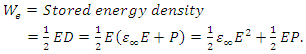(2)

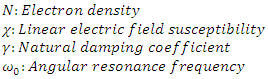
As an example case in which a very high energy can be stored inside a cavity, involves a dispersive medium, which has a frequency dependent permittivity as stated below [5]

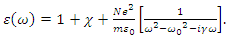(3)

If then we can write [2]

(4)

Assume that there are two monochromatic waves propagating inside a dispersive medium that is placed between two highly reflective walls, and . Let us assume that the angular frequency of is almost equal to the resonance frequency of the medium then the stored energy in this cavity becomes extremely high. Now assume that has a significantly different frequency than the resonance frequency of the medium. Unless it has a very high power, will not yield a noticeable energy increase in the cavity as it’s frequency is not almost equal to the resonance frequency. 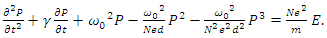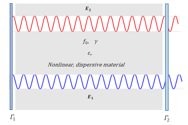Furthermore, will not be able to absorb any energy from the energized cavity as there is no energy coupling mechanism, simply because the medium is linear. To account for an energy transfer from an energized cavity to a low power wave, we need a nonlinear wave propagation analysis between the cavity walls, and for nonlinearity to arise, either the medium itself must be highly nonlinear, or at least one of the waves that propagate inside the cavity must have a very high amplitude.

Figure 1. A cavity with a high electric energy density (due to ) and two propagating waves

3. Wave Propagation in Nonlinear Dispersive Media

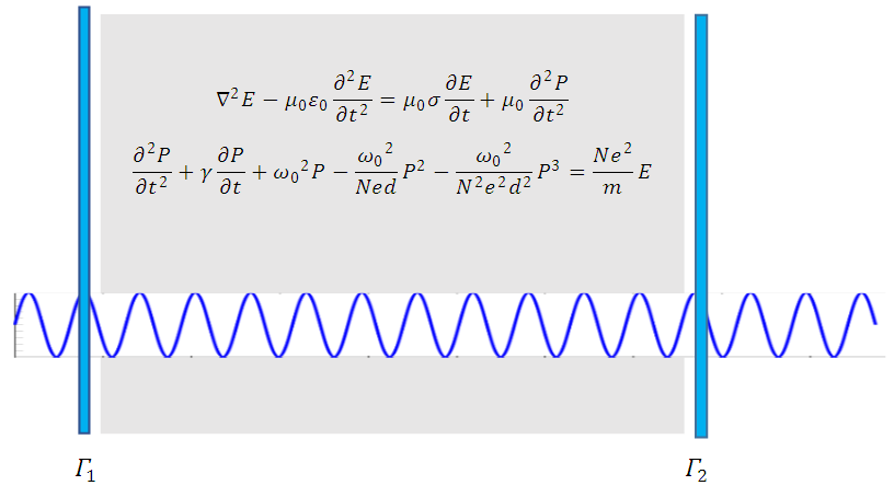
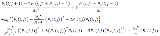
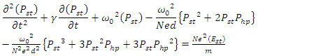
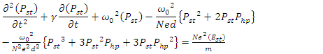
Nonlinearity arises when at least one of the waves that propagate in a medium have a very high intensity. Such high intensities are only possible with very short duration pulses [6,8], such as the pulses of a mode locked laser, which have durations on the scale of picoseconds or femtoseconds [7,9,10]. When high intensity pulses have very short durations, which is almost always the case, we have to account for the wave dispersion, as the impulse response of the charge polarization density of many dielectric media last much longer in duration than the pulse durations of such high intensity pulses.

One can solve the wave equation in parallel with the nonlinear equation of motion of the electron cloud for a nonlinear dispersive medium. This is because the parameters such as the resonance frequency, damping coefficient, atom density, and atomic diameter have known values for most solids, which makes the simulation results much more meaningful and precise. In order to determine the time variation of the electric field in a nonlinear dispersive medium, we need to solve the following two equations [1]:

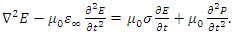(5)

(6)

In Eq. (6) we have made an expansion up to the third order of the nonlinear charge polarization density as higher order terms will be negligibly small. For a dielectric medium, the electrical conductivity can be assumed as negligible Some typical values for solid dielectric media are [1]

Figure 2. A nonlinear dipersive medium placed in a cavity

Consider the wave that has a very high amplitude, without the presence of the low amplitude wave , the pair of equations that describe the propagation of in a nonlinear dispersive medium is given as

(7a)

(7b)

Now assume that and are propagating together in the same nonlinear dispersive medium, in this case the pair of equations that represent the total electric field propagation is given as

(8a)

(8b)

We want to determine the propagation of the low amplitude wave in the presence of the high amplitude wave , in other words we want to determine the propagation of when there is an energy coupling from as a result of the nonlinear interaction. In order to do that we subtract equations (7a,7b) from equations (8a,8b) respectively, which gives us

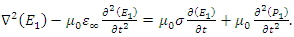(9a)

(9b)

From equations {(7a,7b),(9a,9b)} we can see that and are coupled to each other. Based on equations (9a,9b), we will investigate whether it is possible to amplify the low power electric field , by drawing energy from a low loss cavity that is energized by the high power electric field .

Figure 3. Two waves are propagating through a nonlinear dipersive medium placed in a cavity

3.1. Finite Difference Time Domain Formulation of Energy Coupling in a Nonlinear Dispersive Medium

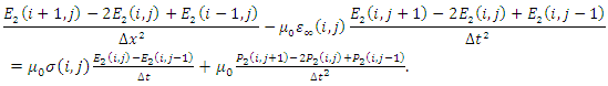
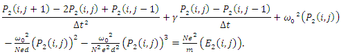
As introduced in the previous section, is the high power wave that initiates the nonlinear energy coupling process and is the low power wave that will absorb energy from . The finite difference time domain formulation of this process in a low-loss dispersive cavity requires the discretization of equations (7a,7b) and (9a,9b). Here we assume a one dimensional space along the x direction so that

(10)

As in every computational problem that has an open (or reflectionless) boundary, we have to define a perfectly matched layer (PML) that must effectively surround and limit the computational region due to memory restrictions [17,18]. Since we are carrying out a one dimensional simulation, there is no issue of precise surrounding of the computational region by the PML. A PML is an artificial region and it surrounds the entire computational domain in order to absorb reflections [20,21]. By minimizing reflections, a PML allows us to obtain realistic results in a limited computational domain of a given problem. One method of realizing a PML is to define a conductivity gradient, by which we assign a zero conductivity at the computational domain interface of the PML, and we gradually increase the conductivity towards the outer PML boundary. Based on Fig. 4 the conductivity gradient that represents the PML region is defined as follows:

(11a)

(11b)

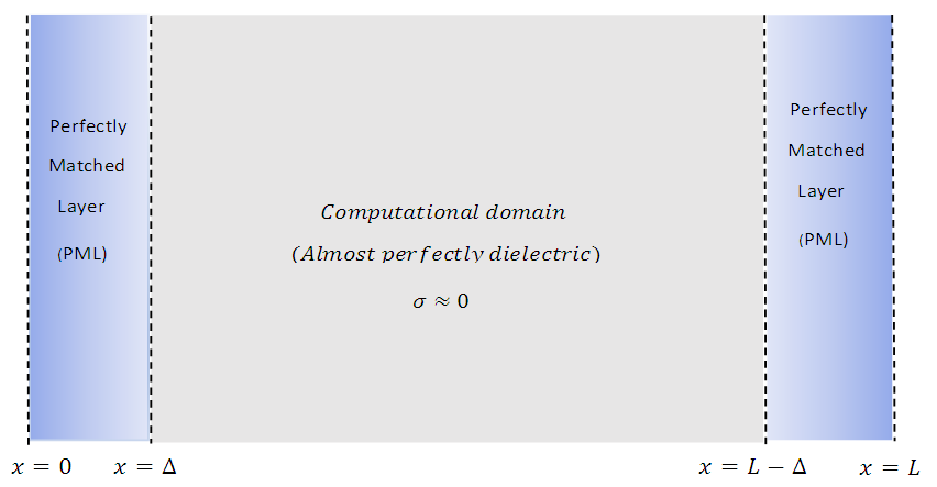Figure 4. The domain of computation and the domain of termination (PML region)

In order to match the intrinsic impedance of the PML region, to the intrinsic impedance of the computational region, we equate their permittivities and permeabilities at the junctions

(12a)

(12b)

(13a)

(13b)

(13c)

(13d)

Having the PML regions of our problem defined based on equations {(11a,11b),(12a,12b),(13a-13d)}, we can now discretize equations (7a,7b) and (9a,9b) using the finite difference time domain method. Let us first discretize equations (7a,7b) as follows:

(14)

(15)

Our aim is to solve for i.e. the value of at a given point at the next time step. Since is coupled to we first solve for and then substitute it into the equation for . We keep on solving these two equations iteratively for all time steps and for all points in the spatial domain of a given one dimensional problem. For a higher accuracy of the resulting solution, we choose and as small as possible [19,20]. Now we discretize equations (9a,9b) and substitute the value of obtained from equations (7a,7b)

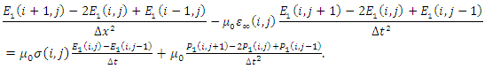(16a)

(16b)

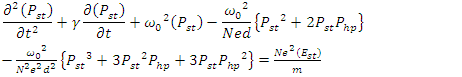
By solving these four equations simultaneously, along with the initial condition and the boundary conditions of a given problem, we can get the time variations of and at any point in one dimensional space. In order to test our computational model, we have compared our computational results with the theoretical results in the well established context of nonlinear sum frequency generation in the appendix section. Now we move on to the simulation results.

4. Simulation Results

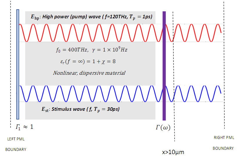
Simulation 1 - Part 1: Sweeping the pump wave frequency to maximize the intracavity energy density

Assume that a 250THz infrared stimulus wave and a high power pump wave (frequency to be determined) are propagating inside a low-loss (high Q) cavity that has two reflecting walls. 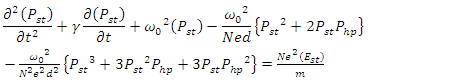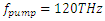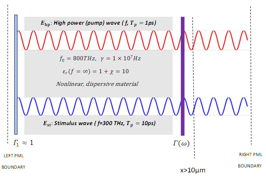The reflecting wall on the left side can be thought as an optical isolator and has a reflection coefficient of the one on the right side represents a switch controlled optical band-pass filter with a frequency dependent reflection coefficient Both waves are generated at x=0𝜇m and at the time instant t=0. The waves and the parameters of the gain medium are as given below:

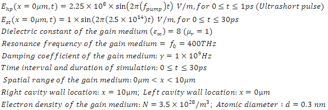
Figure 5. Configuration of the cavity and the dielectric material specifications for simulation1-part1

During the whole simulation time, for all The filter is used for post-processing of the results.

Our problem: Find the optimum pump wave frequency that maximizes in the cavity,

for 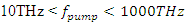(THz to UV), for such that

(7a)

(7b)

(9a)

(9b)

Initial conditions:

Boundary and excitation conditions:

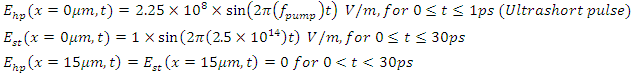Absorbing boundary condition (perfectly matched layer):

Optical isolator condition: Full reflection at

Switch controlled optical bandpass filter condition: Full reflection at for t≤30 picoseconds, frequency dependent reflection at after t=30 picoseconds;

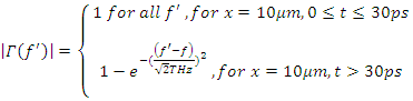If amplified, the stimulus wave at t=30 picoseconds will not be monochromatic anymore, this will be due to the spectral broadening inside the cavity [11-13]. However, by adjusting the center frequency of the band-pass filter to be 250THz, we will get an amplified quasi-monochromatic output. The pump wave frequency will be varied from 10THz to 1000THz in 10THz increments and a pump wave frequency that yields a strong amplification of the stimulus wave will be chosen. 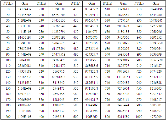The electric energy density and the charge polarization density created by the pump wave, are plotted with respect to the pump wave frequency in Fig. 6 and Fig. 7 respectively. Stimulus wave amplitude gain versus pump wave frequency plot is shown in Fig. 8.

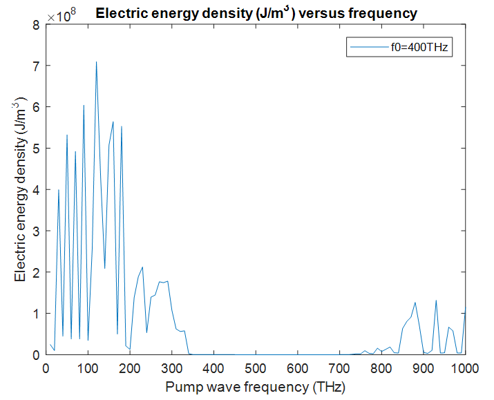Figure 6. Maximum electric energy density created by the pump wave (for 0<t<30ps), as measured inside the cavity at x=5.73µm, versus the frequency of the pump wave

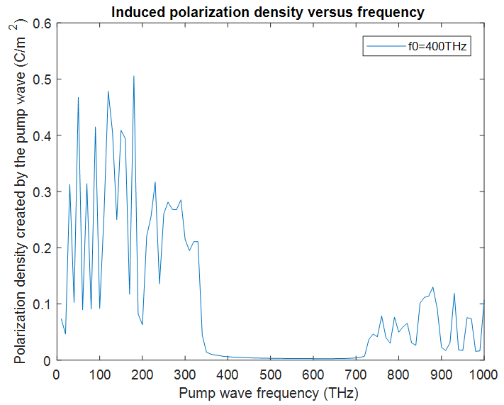Figure 7. Maximum charge polarization density created by the pump wave (for 0<t<30ps), as measured inside the cavity at x=5.73µm, versus the frequency of the pump wave

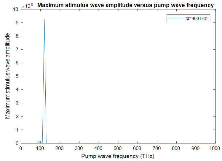Figure 8. Maximum stimulus wave amplitude between 0<t<30ps, as measured inside the cavity at x=5.73µm, versus the frequency of the pump wave

The maximum amplitude of the stimulus wave, versus pump wave frequency plot is shown in Fig. 8. Let us investigate the major amplification peak of the stimulus wave at The peak polarization density created by the pump wave (which acts as the coupling coefficient), is high at this frequency. The peak electric energy density created by the pump wave is also high at Therefore we have an amplification peak at The same is true for all other peaks. If we have a look at Table 1, wherever the electric energy density and the polarization density created by the pump wave, are high, there is a stronger stimulus wave amplification.

Table 1. Maximum stimulus wave amplitude (gain), maximum intracavity energy density created by the pump wave, maximum intracavity charge polarization density created by the pump wave, versus frequency of the pump wave. Gain maximizing pump wave frequency is indicated in bold

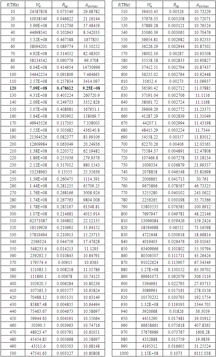
Since the pump wave frequency of maximizes the intra-cavity energy and amplifies the stimulus wave, we choose this frequency as the frequency of pump wave excitation in order to compute the amplification (gain) spectrum of the stimulus wave. However, as already mentioned, the amplified stimulus wave is not monochromatic anymore due to the spectral broadening inside the cavity. Therefore, we must make a seperate analysis to obtain the gain spectrum of the stimulus wave, under a 120THz pump wave excitation.

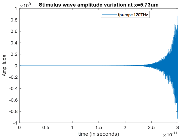Figure 9. Stimulus wave amplitude variation at x=5.73µm for a pump wave frequency of 120THz

Part 2: Investigating the gain spectrum of the stimulus wave for a pump wave frequency of 120THz

Figure 10. The configuration for computing the gain spectrum of the stimulus wave for

Our problem: Under an energy maximizing 120THz pump wave excitation, find the maximum stimulus wave amplitude (gain) in the cavity for each stimulus wave frequency , in the range 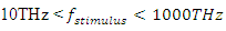(THz to UV), for such that

(7a)

(7b)

(9a)

(9b)

Initial conditions:

Boundary conditions:

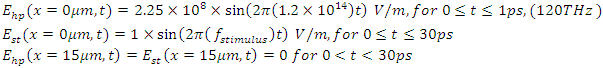Absorbing boundary condition (perfectly matched layer):

Optical isolator condition: Full reflection at

Switch controlled optical bandpass filter condition: Full reflection at for picoseconds, frequency dependent reflection at after t=30 picoseconds. For a given stimulus wave frequency (f), the magnitude frequency response of the filter is chosen to be

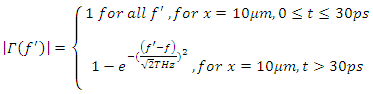The amplification spectrum of the stimulus wave for is tabulated below in Table 2. The stimulus wave is supplied to the cavity at t=0 as a quasi-monochromatic wave. For a given initial (at t=0) stimulus wave frequency, the center frequency of the band-pass filter is adjusted to be at the same frequency with the initial stimulus wave frequency. By doing so, we can observe how much gain can be obtained from the cavity for each initial stimulus wave frequency. We choose the pump wave frequency as as it maximizes the amplification, and we sweep the stimulus wave frequency from 10THz to 1000THz in 10THz increments.

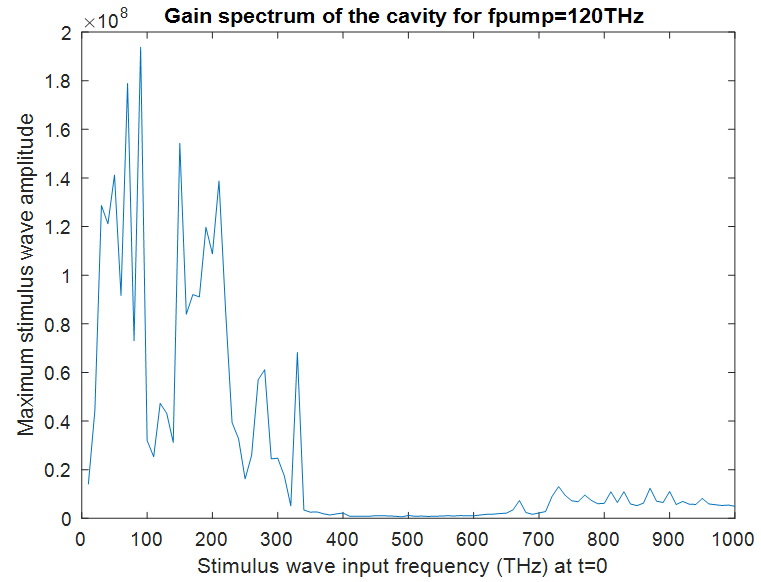Figure 11. Gain spectrum of the stimulus wave for and

Table 2. Gain spectrum of the stimulus wave for       and

Simulation 2:

Part 1: Sweeping the pump wave frequency to maximize the intracavity energy density

Assume that a 300THz infrared stimulus wave and a high power pump wave (frequency to be determined) are propagating inside a low-loss (high Q) cavity that has two reflecting walls. The reflecting wall on the left side can be thought as an optical isolator and has a reflection coefficient of the one on the right side represents a switch controlled optical band-pass filter with a frequency dependent reflection coefficient Both waves are generated at x=0𝜇m and at the time instant t=0. The waves and the parameters of the gain medium are as given below:

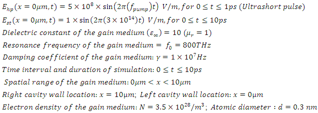
Figure 12. Configuration of the cavity and the dielectric material specifications for simulation2-part1

During the whole simulation time, for all The filter is used for post-processing of the results.

Our problem: Find the optimum pump wave frequency that maximizes in the cavity,

for (THz to UV), for such that

(7a)

(7b)

(9a)

(9b)

Initial conditions:

Boundary and excitation conditions:

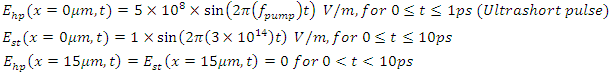Absorbing boundary condition (perfectly matched layer):

Optical isolator condition: Full reflection at

Switch controlled optical bandpass filter condition: Full reflection at for picoseconds, frequency dependent reflection at after t=10 picoseconds;

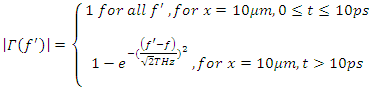If amplified, the stimulus wave at t=10 picoseconds will not be monochromatic anymore, this will be due to the spectral broadening inside the cavity. However, by adjusting the center frequency of the band-pass filter to be 300THz, we will get an amplified quasi-monochromatic output. The pump wave frequency will be varied from 10THz to 1000THz in 10THz increments and a pump wave frequency that yields a strong amplification of the stimulus wave will be chosen. The electric energy density and the charge polarization density created by the pump wave, are plotted with respect to the pump wave frequency in Fig. 13 and Fig. 14 respectively. Stimulus wave amplitude gain versus pump wave frequency plot is shown in Fig. 15.

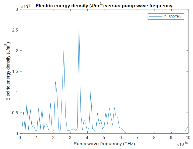Figure 13. Maximum electric energy density created by the pump wave (for 0<t<10ps), as measured inside the cavity at x=5.73µm, versus the frequency of the pump wave

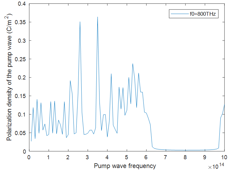Figure 14. Maximum charge polarization density created by the pump wave (for 0<t<10ps), as measured inside the cavity at x=5.73µm, versus the frequency of the pump wave

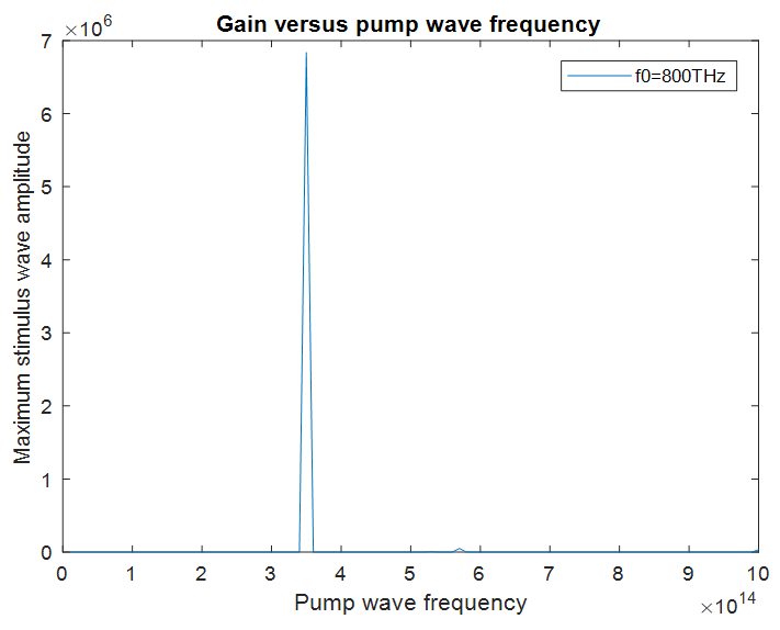Figure 15. Maximum stimulus wave amplitude between 0<t<10ps, as measured inside the cavity at x=5.73µm, versus the frequency of the pump wave

The maximum amplitude of the stimulus wave, versus pump wave frequency plot is shown in Fig. 15. Let us investigate the major amplification peak of the stimulus wave at The peak polarization density created by the pump wave (which acts as the coupling coefficient), is high at this frequency. 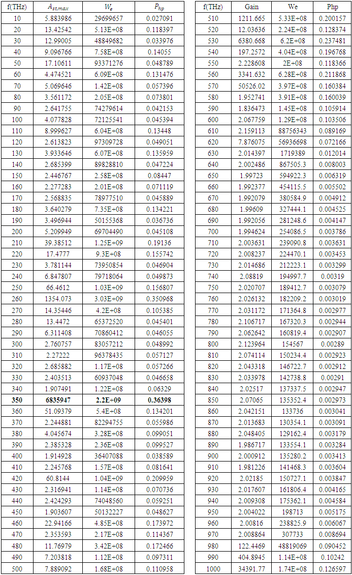The peak electric energy density created by the pump wave is also high at Therefore we have an amplification peak at The same is true for all other peaks. If we have a look at Table 3, wherever the electric energy density and the polarization density created by the pump wave, are high, there is a stronger stimulus wave amplification.

Table 3. Maximum stimulus wave amplitude (gain), maximum intracavity energy density created by the pump wave, maximum intracavity charge polarization density created by the pump wave, versus frequency of the pump wave. Gain maximizing pump wave frequency is indicated in bold

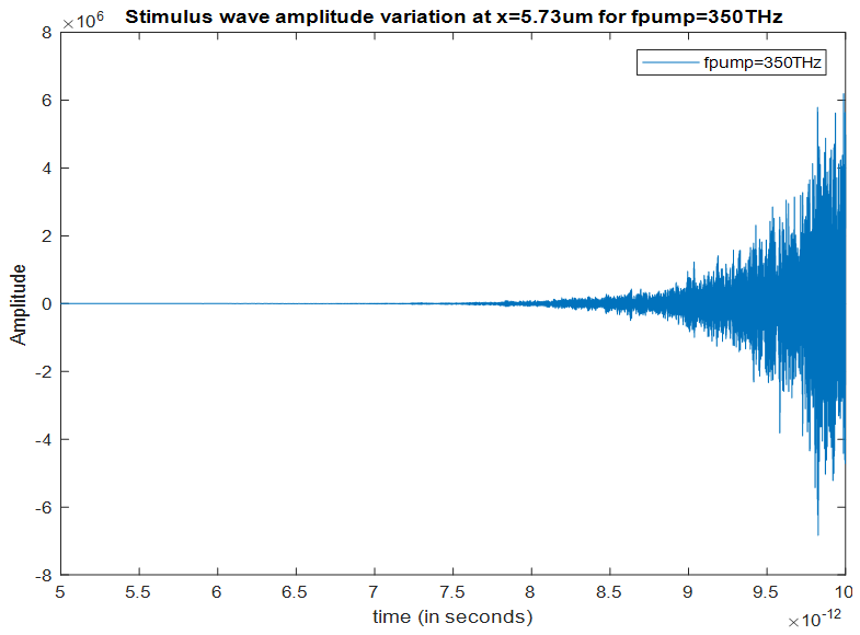Figure 16. Stimulus wave amplitude variation at x=5.73µm for a pump wave frequency of 350THz

Since the pump wave frequency of maximizes the intra-cavity energy and amplifies the stimulus wave, we choose this frequency as the frequency of pump wave excitation in order to compute the amplification (gain) spectrum of the stimulus wave. However, as already mentioned, the amplified stimulus wave is not monochromatic anymore due to the spectral broadening inside the cavity. Therefore, we must make a seperate analysis to obtain the gain spectrum of the stimulus wave, under a 350THz pump wave excitation.

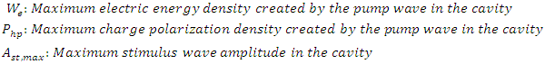Part 2: Investigating the gain spectrum of the stimulus wave for a pump wave frequency of 350THz

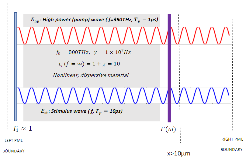Figure 17. The configuration for computing the gain spectrum of the stimulus wave for

Our problem: Under an energy maximizing 350THz pump wave excitation, find the maximum stimulus wave amplitude (gain) in the cavity for each stimulus wave frequency , in the range 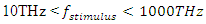(THz to UV), for such that

(7a)

(7b)

(9a)

(9b)

Initial conditions:

Boundary and excitation conditions:

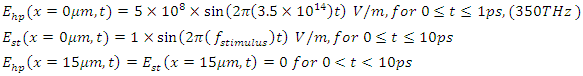Absorbing boundary condition (perfectly matched layer):

Optical isolator condition: Full reflection at

Switch controlled optical bandpass filter condition: Full reflection at for picoseconds, frequency dependent reflection at after t=10 picoseconds. For a given stimulus wave frequency (f), the magnitude frequency response of the filter is chosen to be

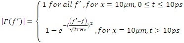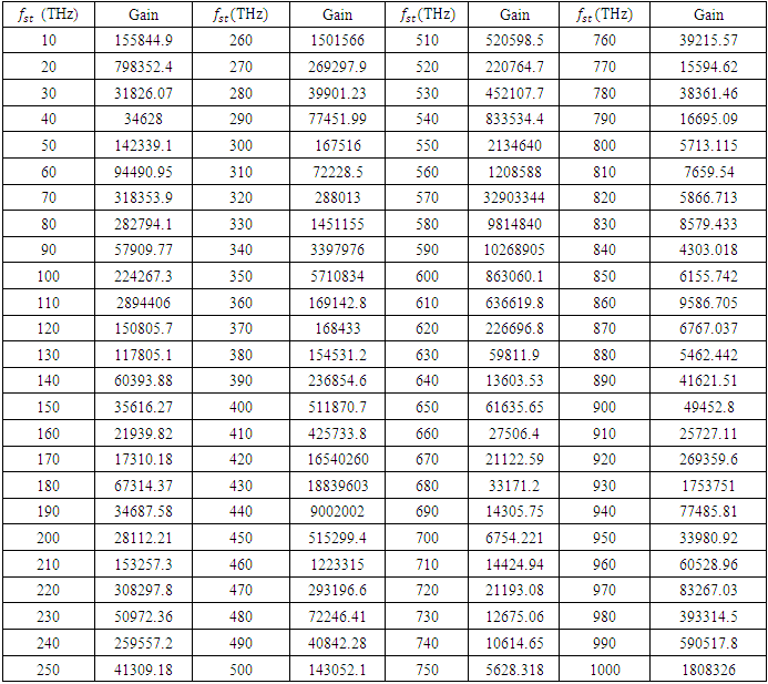
The amplification spectrum of the stimulus wave for 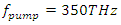is tabulated below in Table 4. The stimulus wave is supplied to the cavity at t=0 as a quasi-monochromatic wave. For a given initial (at t=0) stimulus wave frequency, the center frequency of the band-pass filter is adjusted to be at the same frequency with the initial stimulus wave frequency. By doing so, we can observe how much gain can be obtained from the cavity for each stimulus wave frequency. We choose the pump wave frequency as as it maximizes the amplification, and we sweep the stimulus wave frequency from 10THz to 1000THz in 10THz increments.

Table 4. Gain spectrum of the stimulus wave for       and

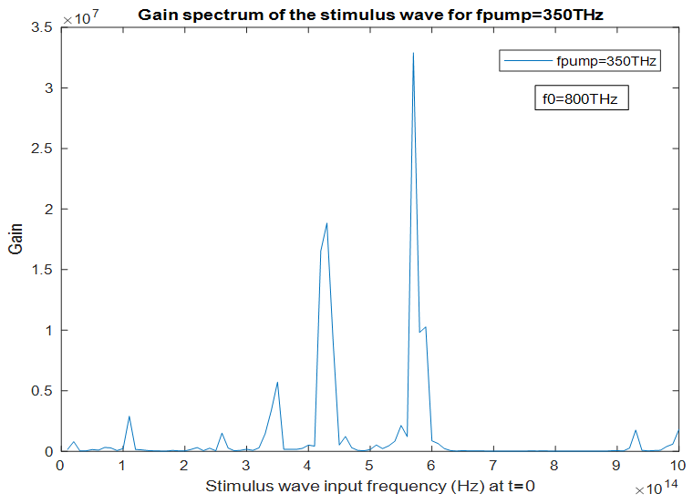Figure 18. Gain spectrum of the stimulus wave for and

5. Conclusions

In order to amplify a low power stimulus wave via nonlinear wave mixing in a low-loss optical microcavity, a high intracavity energy is required. As a summary for intracavity energy maximization and efficient wave amplification, the following requirements should be met:

• The cavity should have a high quality (Q) factor.

• For a given resonance frequency of the material, the high power pump wave frequency must be adjusted to maximize the electric energy density inside the cavity.

Once these requirements are satisfied, it is possible to amplify a low power input wave, with a very large gain coefficient, by mixing it with an intense pump wave of very short duration, in a wide range of frequencies, inside a low-loss optical microcavity.

6. Appendix

6.1. Validation of the Computational Model and Results

In this section, we will compare our finite difference time domain based computational model with the theoretical formula in the well-established context of sum frequency generation via nonlinear wave mixing, in the following example.

Example: Nonlinear sum frequency generation (frequency upconversion)

This example is about the generation of a higher frequency component by mixing of two monochromatic waves with frequencies such that 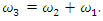In order to achieve this, at least one of the waves must have a high intensity, so that nonlinearity arises, and wave mixing occurs.

The high amplitude pump wave is generated at It has an amplitude of and a frequency of 180THz.

The input wave is generated at It has an amplitude of and a frequency of 120THz.

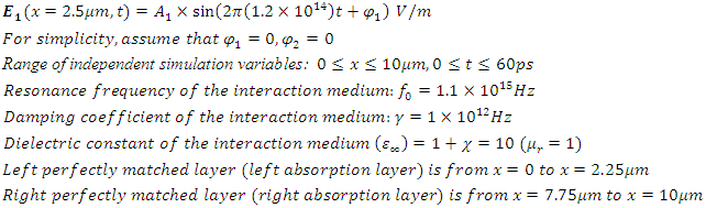
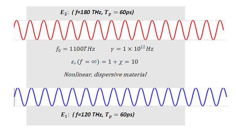Figure 19. Configuration for frequency upconversion

The theoretical formula for frequency upconversion efficiency, which is derived from the solution of nonlinear wave equation that is based on material nonlinearity coefficient, is given as [1,4]

(7)

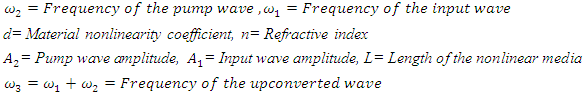Our computational model is based on the finite difference time domain discretization of the nonlinear electron motion equation that involves the resonance frequency and the damping coefficient of the interaction medium. Coupled with the wave equation, the total wave can be evaluated from:

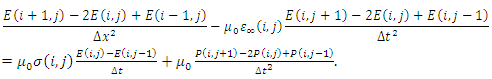(8a)

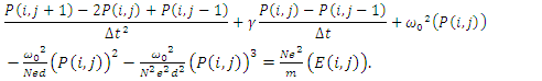(8b)

For a time interval of the computational formula for frequency upconversion efficiency is

(9)

In this example, we have used the following values for each efficiency formula

d= Material nonlinearity coefficient = (The theoretical and the computational results agree for this value of d for a sample pump wave amplitude of Our aim is to see if the results also agree for all the other pump wave amplitudes for this value of d)

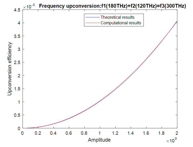Figure 20. Comparison of the frequency upconversion efficiencies for and versus the pump wave amplitude