-
Paper Information
- Paper Submission
-
Journal Information
- About This Journal
- Editorial Board
- Current Issue
- Archive
- Author Guidelines
- Contact Us
International Journal of Electromagnetics and Applications
p-ISSN: 2168-5037 e-ISSN: 2168-5045
2018; 8(1): 1-25
doi:10.5923/j.ijea.20180801.01

Space Mission Analysis and Design for Electromagnetic Suppression of Radar
 Abstract
 Reference
 Full-Text PDF
 Full-text HTML
Timothy Sands
Department of Mechanical Engineering, Stanford University, Stanford, USA
Correspondence to: Timothy Sands, Department of Mechanical Engineering, Stanford University, Stanford, USA.
| Email: |  |
Copyright © 2018 The Author(s). Published by Scientific & Academic Publishing.
This work is licensed under the Creative Commons Attribution International License (CC BY).
http://creativecommons.org/licenses/by/4.0/

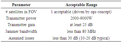
Inspired by aerial combat in the Balkans (Serbia and Kosovo) in 1999 with no known support suppressing enemy air defenses (SEAD) from space, this article proposes such by first introducing the reader to basic electromagnetic principles in order to evaluate the SEAD radar jamming mission from space. Next key design parameters are iterated in physics-based simulations to drive subsequent design efforts. Electromagnetic propagation equations are simulated and iterated to reveal key threshold values of key design parameters. It is revealed that only a single satellite is required for effective jamming with transmitter power of 2-9 kilowatts, transmission gain of at least 25 decibels, while maintaining a bandwidth less than 80 megahertz and assumed losses less than 30 decibels (where 10-20 decibels is typical). Using these key thresholds, space mission analysis and design (SMAD) is articulated in detail for the first time in the literature, revealing rough-order-of-magnitude budgets for system design. The design requires elements of mechanical engineering, electrical engineering, and aerospace/astronautical engineering at least. Astrodynamics reveals that a low-earth orbiting altitudes of 100-400 kilometers produces jamming effects on the target emitter for 4.8-10.2 minutes respectively producing jammer energy received by the targeted radar of -23.9 to -102.9 decibel-watts respectively. These key design features are used to establish a link-budget that reveals mission margin. Spacecraft key design budgets are calculated next revealing the requirement for a large spacecraft (~7333kg, 7.8m X 61.1m2) and large launch vehicle (Atlas V class). Budgets are also found for key satellite subsystems: payload, structures, thermal, power, TT&C, attitude control, and propellant. Reliability calculations and cost estimated are discussed, and normalized evaluation of jamming effectiveness is recommended. Lastly, key technology challenges of target acquisition, tracking, and spacecraft fine pointing are discussed, and current research efforts are highlighted inspiring future directions for technical innovations to enhance the design.
Keywords: Space mission analysis and design, Suppression of enemy air defenses (SEAD), Radar jamming, Electrical engineering design, Aerospace engineering design, Mechanical engineering design
Cite this paper: Timothy Sands, Space Mission Analysis and Design for Electromagnetic Suppression of Radar, International Journal of Electromagnetics and Applications, Vol. 8 No. 1, 2018, pp. 1-25. doi: 10.5923/j.ijea.20180801.01.
Article Outline
1. Introduction
- The nature of the problem goes far back to World War II and continued through the Vietnam War into today and tomorrow. The lessons regarding the critical nature of electronic warfare (EW) to combat operations have been relived repeatedly ever since in the Israeli war of 1967, the Falklands Conflict in 1982, and very recently in Operations DESERT STORM against Iraq and ALLIED FORCE against Yugoslavia. I can speak first hand to the fact that I live today due to a combined electronic warfare campaign waged by multiple systems in a synergistic manner. Lessons discovered during ALLIED FORCE include that American electronic warfare platforms are again at a premium, just like they were at the beginning of the Vietnamese War. The only dedicated EW strike aircraft in all of the military services is the Navy EA-6B Prowler. Against Iraq, the Air Force still operated the EF-111, but retired it before entering the war in Yugoslavia. That left America dependent upon one single Navy plane for defense. This plane was also responsible for Navy fleet defense. Limited jammers struggled to cover the list of critical air assets requiring defense. This research reaffirms the absolute necessity of electronic combat to modern warfare. In light of the shortfall of American electronic warfare aircraft, I intend to aid the U.S. warfighter with satellite based electronic warfare.The following manuscript will step back briefly to explain radar in a section called “electromagnetic (EM) radiation principles.” Then radar jamming will be described in a section called “Electronic Warfare” followed by a brief discussion on the need for comprehensive suppression of enemy air defenses (SEAD). Next, two kinds of jamming are described in a section on “Modulated jamming versus Non-modulated jamming” (these terms will be defined in that section using knowledge from the section on EM radiation principles). Space-based ECM is a complex legal issue. Accordingly, sequential sections cover the legality and political realities of space-based electronic warfare by reviewing the relevant treaties and discussing the politics of such a jammer system in space. The final sections contain engineering analysis to demonstrate real-world feasibility today. Mission design of Space-based ECM is feasible. Radiation analysis demonstrates jamming threat radars from orbit. Then, potential concepts for satellite development are introduced. After lengthy analysis the final product is first order design with engineering development budgets suitable for further education research.
2. Electromagnetic Radiation (EM) Principles [1]
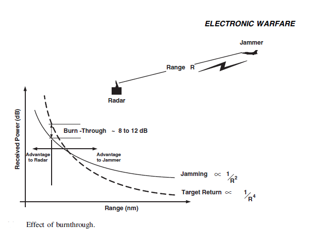
- Electromagnetic energy propagates through space in all directions at the speed of light. It is made up of two sinusoidal waves orthogonal to each other and direction of wave propagation. One wave is electrostatic and the other is magnetic. A jammer transmits EM energy at matching frequencies in hopes of overcoming the return energy per figure 1.
 | Figure 1. Electromagnetic (EM) radiation and jamming burnthrough [2] |
|
|
|
2.1. Electronic Warfare (EW)
- Electronic Warfare begins with matching the enemy’s radar frequency with jamming energy. A key notion of effective EW is continuous interference. If the jamming is not continuous, the enemy will be able to reconcile a firing solution on your aircraft and shoot you from the sky. For this reason, an analysis of how long the spacecraft will be overhead is key. The amounts of time that jamming is available can directly limit safe air combat activities. Another key concept to understand is burn-through range. There is a range at which the return echo of a radar-detected aircraft will be stronger than the jamming interference energy. At that point the threat radar has “burned through” the jamming and can fire on the aircraft. For this reason, it is best to maximize the amount of interference energy to reduce the burn-through range to near the minimum range (to be defined next). To maximize the interference energy, utilize a synergistic application of multiple jammers from any and all directions. This is the essence of modern electronic warfare. This manuscript for space-based electronic countermeasures (ECM) proposes to augment this synergy, not replace any current jammer platforms. Certainly in light of the small amount of ECM platforms in the military arsenal, anything will help. The minimum range just discussed is an inner limit to how close radars can detect target aircraft. As the radar switches from transmit to receive, the receivers are saturated with transmission noise. This is called duplexer-switching time or recovery time. During this time the radar cannot detect incoming aircraft. This time directly correlates to a “radar distance” that it cannot detect aircraft. Since the radar cannot see while it is recovering, this time establishes what is called the minimum range. If jamming energy can be made powerful enough to push the burn-through range back near the minimum range, the radar is defeated.
2.2. Modulated Jamming versus Non-modulated Jamming
- Raising the jamming energy as high as possible is the key to non-modulated jamming (saturate the threat with non-modulated noise). Another approach to jamming is to match the modulation scheme of the threat radar. As previously discussed, threat radars can modulate their signals, then listen for only return echoes that have the correct modulation. This reduces the effectiveness of noise jamming. The threat radar operator may not even have interference until its receivers become saturated. For this reason, jammers should attempt to match the threat emitter’s modulation in addition to its frequency. This manuscript will not discuss any sort of modulations of jamming signals. All analysis applies to non-modulated noise jamming with the assumption that future modifications can easily allow modulated jamming from space.
2.3. Legality of Satellite-Based Electronic Warfare
- While not widely publicized, electronic warfare from space is not a new idea. In the 1989 book, Military Space Forces: The Next Fifty Years, John M. Collins envisioned electronic warfare as “mainly high-power proximity jamming” of other spacecraft in orbit. [3] The ease of electronic jamming in space justifies manned presence in his idea of space warfare, since “spoofing and other forms of electronic warfare could shut down autonomous and remotely controlled systems more readily than those with manual overrides”. [3] To aid Allied war fighting, a joint space-based electronic warfare system (JSBEWS) is proposed in hopes to exploit this ease of jamming. Why this not done much earlier? Certainly the technology existed decades ago to launch satellites and to jam radars from high-flying aircraft. To answer this question, visit the jurisprudence of space. Space law exists in part to prevent conflict in space and must be studied to insure the legality of space-based ECM.
2.3.1. Outer Space Treaty (OST)
- The Outer Space Treaty (OST) is regarded by many to be the basis of international space law. It was adopted in 1966, and has been signed by 28 nations and ratified by 92 nations including the U.S. and U.S.S.R. [4]. In the treaty, most of the world’s space faring nations agreed to amongst other things [8]: 1) Not place weapons of mass destruction in orbit around the Earth, on celestial bodies, or in space in any manner (Article 4 OST [6]). 2) Outer space and the celestial bodies are not subject to sovereignty, occupation, or national appropriation (Article 2 OST [7]), and 3) The general principles of liability, registration, and jurisdiction (Article VIII OST [8])Denying the enemy radars a view of incoming Allied warplanes would fall under the label of “Information Blockade” in Space Power 2010 by researchers at the Air Force’s Air Command and Staff College. [5] The paper also states that “although the Outer Space Treaty does limit military and industrial activities in space, it alone does not prohibit the achievement of the space power CONOPS (Concept of Operations)” which contains Information Blockade [5]. This must include a favorable interpretation of Article III, which states (emphasis added) [6]:“States Parties to the Treaty shall carry on activities in the exploration and use of outer space, including the moon and other celestial bodies, in accordance with international law, including the Charter of the United Nations, in the interest of maintaining international peace and security and promoting international cooperation and understanding.” So, it seems that in some cases it would be acceptable to have overhead jamming of threat radars. It must be in accordance to international law (which does not prohibit all war) and the Charter of the United Nations (which allows for the use of force to maintain peace). Operation DESERT STORM and perhaps even NATO Operation Allied Force seem to fit the criteria above implying space-based jamming could have been used legitimately.
2.3.2. Moon Treaty
- The Moon Treaty was adopted in 1979 with 11 signatory countries and 9 ratifications, not including the U.S. or U.S.S.R. [4] It reiterates the principles in the Outer Space Treaty and adds details of prohibited military acts in space. Utilizing customary law, it is useful to examine the Moon Treaty as a likely precedent for restrictions of military activities in orbit. The Moon Treaty specifically prohibits “any threat or use of force or any other hostile act or threat of hostile act on the moon” (Article 3) [6]. Article 4 specifies “The use of military personnel for scientific research of for any other peaceful purposes shall not be prohibited”. [6] Having earlier established that some wars will be fought to obtain peace and will be sanctioned by the United Nations. A military Electronic Warfare Officer could legally ride aboard the Space Shuttle to operate radar-jamming equipment during sanctioned conflict. This would not be prohibited by the Outer Space Treaty and is also consistent with the details of the Moon Treaty details.
2.3.3. The ABM Treaty Reinterpretation [6]
- The Anti-Ballistic Missile (ABM) Treaty took effect in 1972 and codified the limits of testing and deployment of such systems that could track, intercept and destroy incoming ballistic missiles. In 1985, the Reagan administration created a new legal interpretation of the treaty to allow the United States to begin full-scale testing of space-based lasers and other advanced weapons. The Treaty does not apply any restrictions to space-based jamming of threat radars, and there were many arguments against this reinterpretation. The example cited here is how far the reinterpretation of international law has already come: to the extent that weapons may be put into space (examples in the next section). Perhaps it will not be so difficult to ‘sell’ electronic warfare from space after all. If weapons were already nearly put in space, electronic interference equipment should be much easier to justify. What is the exact definition of a space weapon? Does it include electronic warfare equipment?
2.3.4. Define Space Weapon (Weaponization of Space) [7]
- The 1996 National Security Strategy of Engagement and Enlargement calls orbiting space weapons a deterrent and a substitution for overseas presence. [8] Space weapons are defined functionally as disrupting, degrading, denying, or destroying an adversary’s assets in any medium. A study by Air University directed by Air Force Chief of Staff General Fogelman elaborated on the concepts and capabilities of US space weapons. The study focused on three categories of space activities: space strike weapons, space guided weapons, and information warfare. Space strike weapons included directed energy weapons like lasers that strike targets offensively. Space guided weapons include precision guided munitions using Global Positioning System (GPS) amongst other concepts. These space weapons already exist today, so a very strong argument could be made that the weaponization of space has already occurred. Electronic Warfare is an example of Information Warfare as defined by the Air University study. This study takes the position that electronic warfare constitutes space weaponization since it is a kind of Information Warfare. According to Maj Gen Harry Raduege USAF Command, Control, Communications, and Computers Systems are now classified as weapon systems. Maj Gen Raduege is a former Director of NORAD/USSPACECOM/AFSPACECOM Information Systems. Up until recently, Information Warfare (IW) was not considered a classical weapon system. “Since these are not guns or bullets, by the definition they are not space weapons. Thus, IW (which includes electronic warfare) does not weaponize space”. [8] A space weapon is defined by its offensive nature and intent to cause harm. By either logic, we have already weaponized space with GPS guided bombs and missiles. There have also been weapon platforms put directly into orbit. The Soviet Union orbited a Fractional Orbital Bombardment Systems (FOBS) designed to drop nuclear bombs on America from orbit. [9] Additionally, the United States deployed an anti-satellite weapon system (Program 437) for 10 years in 1965. [9] Arguing the strong case in favor of JSBEWS, Electronic Warfare is not even considered a space weapon. Arguing the devil’s advocate position against JSBEWS, the strictest interpretations would include EW as a space weapon. But, since it lacks the offensive nature of pre-existing space weapons, customary law would allow space-based electronic warfare even under this devil’s advocate position. JSBEWS should be legally defensible.
2.4. The Politics of Satellite-Based Electronic Warfare
- JSBEWS is legally defensible, but what about the political realities? Politicians decide such matters regarding national defense and national security.“Negation, or offensive counter-space, is the space control mission in which the operational commander has his broadest latitude and greatest capability. Destruction, denial, and deception are the principal military methods to negate space systems. Recent DOD strategy reflects an important shift toward a more politically realistic approach to space negation—extending space control beyond the realm of direct attack on celestial assets, to attacking ground stations, interfering with satellite uplink and downlink signals, and applying diplomatic influence to limit access to space-based systems.” [10] Electronic warfare here specifies jamming satellite uplink and downlink signals, but the point remains. Today’s political reality is moving away from physically destructive space strike systems into electronic warfare, since it is more politically palatable. Information Warfare is the wave of the future. To deny the enemy information increases his fog during war. [9] JSBEWS could provoke anti-satellite countermeasures, but that is unlikely. The ubiquitous use of GPS weapon guidance has not provoked such activity. The main point of this discussion of politics has been that space-based electronic attack is far easier to legally justify than today’s destructive space weapons. After demonstrating that this system is legal and also politically palatable, the following sections describe a first order engineering design of JSBEWS. Equations were elaborated and explained where it seemed that such an explanation would help the reader understand the system best. There is absolutely no way to elaborate on every calculation made (as will become quickly obvious). Therefore the remaining equations are cited with page number and even equation numbers to allow the skeptics to check the work.
2.5. Supression of Enemy Air Defenses (SEAD) from Space
- Electronic warfare from space begs the question, “Isn’t space too far away?” The air defense engagement is analyzed in depth. Using a baseline transmitter, burnthrough ranges are used to iterate specific design parameters of the spaceborne jammer. This work is certainly not comprehensive, but suits its purpose by initiating conversation of space based electronic warfare with some hard-hitting calculations. The electronic engagements are analyzed in too-great detail for plug-and-chug equations. Instead, computer simulation is used with some explanations to give the reader an understanding of the factors taken into account. The reader will immediately note that this paper will strictly discuss noise interference jamming with a baseline spacecraft versus a nominal C-band surface-to-air missile system (SAM). Do not mentally extrapolate the results in this paper to newer SAMs.A typical RADARSAT remote sensing mission maps the earth using very tightly focused radar energy. The reader is encouraged to consider a threat radar emitter on the earth under one of the patches illuminated by the remote sensing radar. For jamming purposes, the radarsat would not push-broom sweep the earth. Instead the spacecraft must maneuver to constantly keep the spot beam of energy focused on a geographic point on the earth as it flies overhead. This will eventually drive the need to discuss target acquisition, tracking, and spacecraft fine pointing. Key parameters for first-looks at electronic warfare engagements often begin with the slant range. For jamming from space, accounting for the spherical earth is absolutely necessary to find the slant range and the time-in-view. Recall the satellite is flying by in (an assumed) low-earth orbit (LEO), so jamming is definitely limited to some small amount of time. The electronic engagement is simulated to reveal key jammer design parameters for space based electronic warfare. The “bible” for this analysis is ref [11] with additional significant references provided.Satellite electronic attack on enemy air defense radars is a pioneering use of orbiting radar emitters that were once used for remote sensing. Electronic attack is not the same as remote sensing, so a detailed design analysis of candidate space radar systems is required. The Shuttle Radar Topographic Mapper Mission (SRTM) seems perfectly capable of electronic attack based upon ongoing engineering analysis. The electromagnetic propagation path is narrowly evaluated to answer the basic critique, "Isn't space too far away". This evaluation establishes critical limits for key parameters: 1) number of satellites required in the enemy’s field of view, 2) transmitter power, 3) transmitter gain, 4) transmitter bandwidth, and 5) assumed losses resulting in burnthrough ranges for various assumed design parameters.
2.5.1. Electromagnetic Engagement Simulation
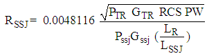
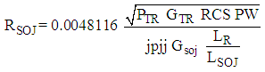
- Since the equations necessary to truly examine the electronic battlefield can become burdensome, computer simulation is mandated. The core of the simulation model is derived from [12]. The basis of the simulation model is the self-screening and the support jammer burn through equations. The equations are written and described here in typical textbook terms [13]-[19] for easy understanding. The support or stand-off jammer burn through equation is:
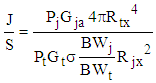 | (1) |
|
 | (2) |
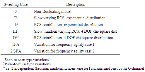
2.5.2. Swerling Model
- A method to mathematically model radar cross-section fluctuations is using the Swerling cases, sample, generic cases developed by Professor Swerling. Swerling case I assumes the target RCS is constant during the duration of a scan, but varies from scan-to-scan. Swerling case II assures the target RCS varies from pulse-to-pulse. The kinds of models include the five Swerling cases 0 through 4 with the non-fluctuating model indicated by Swerling 0. Swerling Case 3 and 4 targets are random variables drawn from a chi-square distribution having four degrees of freedom while Swerling Case 1 and 2 targets are drawn from an exponential distribution (i.e. two independent Gaussian random numbers, one for the I channel and one for the Q channel). Swerling 1 and 3 targets are slowly varying targets, fluctuating from scan to scan, while Swerling 2 and 4 exhibit pulse to pulse type fluctuations. The temporal decorrelation effects are handled the same way for both fast and slow fluctuating targets. The target pulse values are passed through a second order IIR filter whose filter coefficients are derived with Gaussian assumption. The Gaussian value is 1 PRI for the decorrelation time (time to de-correlate to 1/e) for fast fluctuating targets (Swerling 2 and 4) and 1 second for slow fluctuating targets (Swerling 1 and 3). This is all accounted for in the portion of the simulation model called “delectability factors” for the seven cases. They are broken into the following seven delectability factors accounting for their respective swerling case with mathematical simplification:det_facts(1)=snr_noncoh_detdet_facts(2)=snr_noncoh_det + W * fluct_lossdet_facts(3)=snr_noncoh_det + W * fluct_loss/non_coh_pulsesdet_facts(4)=snr_noncoh_det + W * fluct_loss/2det_facts(5)=snr_noncoh_det + W * fluct_loss/(2*non_coh_pulses)det_facts(6)=snr_noncoh_det + W * fluct_loss/N_expdet_facts(7)=snr_noncoh_det + W * fluct_loss/(2*N_exp)There are seven options resulting in seven burn through ranges. Warfighters really need a single average answer to make meaningful decisions, so the matrix has been averaged to yield a single burnthough range number. Both of these results are provided by the simulation graphically: 1) Average burn-through number, and 2) Seven Swerling case burn-through numbers.
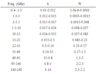
2.5.3. Variables and the Range of Variation
- Radar transmitter power: ≤~5 MWRadar Frequency: 400 MHz-240 GHzPulse width: VariesJammer and threat radar gains: ~0-45dBPulse repetition frequency: 0-500,000Signal bandwidth ~10-200 MHzAtmospheric/propagation losses: VariesGains and losses: system noises ~ -10-10 dBDoppler bandwidth: ~100’s HzFrequency agility bandwidth: ~100’s MHz Azimuth bandwidth: ~couple of degeesAzimuth rate: ~tens of degees/secondOrbit height: ~100’s of km for LEO
2.5.4. Fixed Parameters: Simulation Input Assumptions
- Probability of detection: ≡ 90%Probability of false alarm: ≡ 1e-6Target radar cross section: 0.1Target elevation angle: <1o, let 0.4oTarget length: 10mRadius of earth: 6378.14 kmRain fall rate: Let 0 for this simulationFrequency dependent atmospheric attenuation:
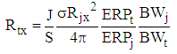
2.5.5. Mathematical Expressions
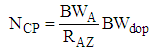
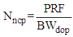
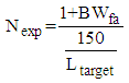
- Several mathematical expressions are required enroute calculations. These expressions model physical aspects of the equipment used on both sides of the air defense scenario. Nominal range index (lacking jamming), system noise, number of independent, coherent, and non-coherent pulses, and the mathematical programming expressions of the burn through equations are listed next.Nominal Range Index (no jamming):
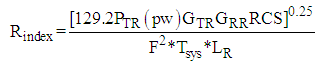 | (3) |
 | (4) |
 | (5) |
 | (6) |
 | (7) |
2.5.6. Logical Statements Defining the Properties of the Model or Solution
- The effects of jamming must be accounted for with logical programming code to allow combinations of 1) self-screening jamming only, 2) stand-off jamming only, and 3) both self-screening and stand-off jamming. The self-screening and stand-off jamming options are established in separate files then combined with logical programming code to allow all three options. The simulation was run iteratively for various parameters revealing nominal values of each parameter. Nominal values were assumed and then each parameter was iterating individually with results summarized in the next section. Self-screening jamming burn through range:
 | (8) |
 | (9) |
2.5.7. Simulation Results
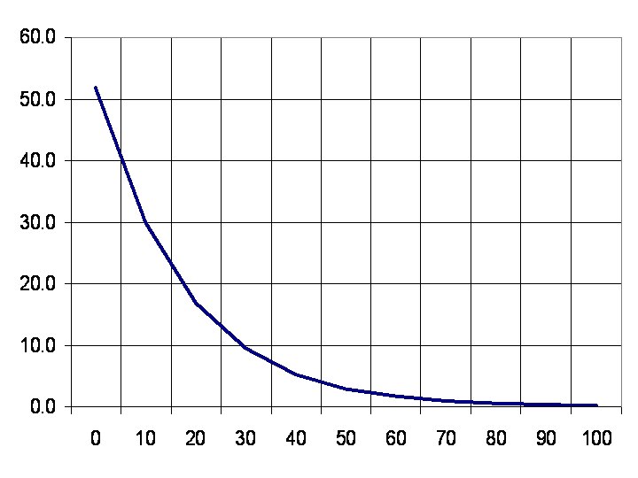
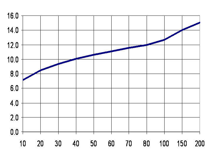
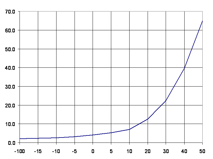
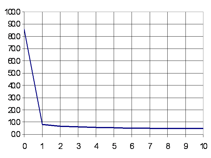
- In considering the utility of satellite radio-frequency emitters for electronic attack of enemy air defense radars, operator and designers alike need to understand useable ranges of key design parameters like jammer transmitter power, gain, bandwidth, assumed losses, and the minimum number of required satellites. Simulations reveal iterations of these key design parameters. Figures 2-6 display the results. One first key point to note is demonstrated feasibility of the concept of electronic attack from satellites. The SRTM radar spacecraft flown in 1999 seems capable of providing appreciable burn-through ranges against C-band surface to air missiles with a targeted aircraft of 1 m2 radar cross-section. Figure 2 reveals the nominal SRTM transmitter operating power (3000-9000W) provides ample burnthrough range assuming noise jamming. Next, Figure 3 reveals the required gain establishing 20-40 dB antenna gain as a key design limit. Figure 4 reveals that transmitter bandwidths are important and illustrate that tighter bandwidth requirements result in superior burn-through range. Figure 5 exposes particular vulnerability to assumed losses. Losses must be kept lower than ~20dB, since performance is dramatically decreased beyond this limit.
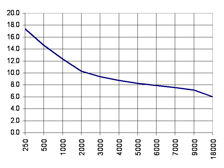 | Figure 2. Burnthrough (miles) versus SA-2 surface-to-air missile radar for assumed 1m2 targeted aircraft for various transmitter antenna power (W) |
 | Figure 3. Burnthrough (miles) versus SA-2 surface-to-air missile radar for assumed 1m2 targeted aircraft for various transmitter antenna gains (dB) |
 | Figure 4. Burnthrough (miles) versus SA-2 surface-to-air missile radar for assumed 1m2 targeted aircraft for various transmitter bandwidths (MHz) |
 | Figure 5. Burnthrough (miles) versus SA-2 surface-to-air missile radar for assumed 1m2 targeted aircraft for various assumed signal strength losses (dB) |
|
 | Figure 6. Burnthrough (miles) versus SA-2 surface-to-air missile radar for assumed 1m2 targeted aircraft for various numbers of satellites in enemy radar field of view |
2.5.8. Summary of Key Design Parameter Values
- This section reveals the fundamental questions considering space based electronic warfare: 1) Can you actually launch a satellite big enough to perform it (as determined by the requirements of jammer power and antenna gain), and 2) Isn’t space too far away. The first question is addressed by assuming a nominal jammer transmitter power of 3000W. Detailed analysis and simulation of the electromagnetic engagement revealed that a SIR-C/SRTM type radar in a Space Shuttle orbit can achieve appreciable burnthrough range for an assumed 1m2 targeted strike aircraft versus a C-band SAM with realistic assumed parameters. These values inform the next step: Space Mission Analysis and Design (SMAD).
3. Results: The Engineering Design
- So far it has been demonstrated that Space-based Electronic Countermeasures against threat radars is highly desirable and legally and politically feasible. A question which remains is, “Is it technically feasible with the state of today’s technology, or is SBEWS a dream for the future?” The next sections will address this with engineering analysis to verify that indeed radars can be jammed from orbit. The first section is called “Orbital Parameters” and it lays out the terms used in the initial analysis. The next two sections, “Radar Energy Received by Threat Emitter” and “Link Analysis” will first use the radar equation (to be defined) and then a detailed link analysis to verify that the energy received at the ground threat radar is sufficient to jam it. After showing that space-based jamming is possible, the next section estimates the scope of a free-flyer jammer satellite. The section is called “First Design Choice: System Scope.” Several sections after that include preliminary engineering design arriving at initial engineering budgets. Finally, a discussion of the space-based jammer design evaluation is followed by itemized cost estimation for the system. This all makes sense with a common understanding of some basic terms, beginning with orbital parameters.
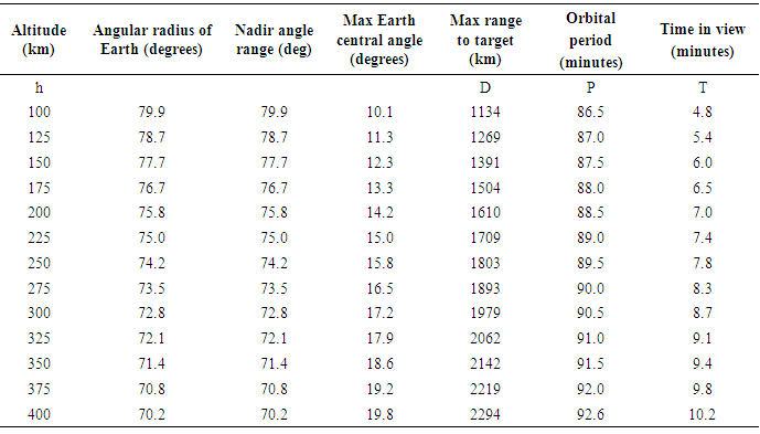
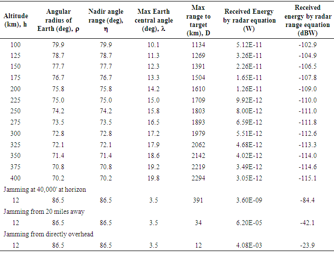
3.1. Orbital Parameters
- Referencing figure 7, The Space Shuttle’s orbit is a likely starting place for analysis. This selected orbit of 185 miles (roughly 300 km) [11] circular yields an angular radius of earth:
 | (10) |
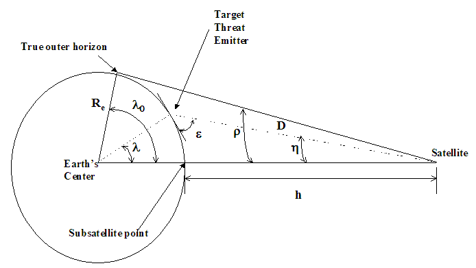 | Figure 7. Geometric relationships |
 | (11) |
 | (12) |
 | (13) |
 | (14) |
|
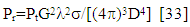
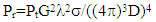
3.2. Radar Energy Received by Threat Emitter
- Now that the max slant range to the target is known, the radar range equation can reveal the received power given a typical transmitted power. Along the way, satellite design parameters will become established, but first briefly summarize. The radar equation is
 | (15) |
 | (16) |
 | (17) |
 | (18) |
|
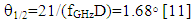
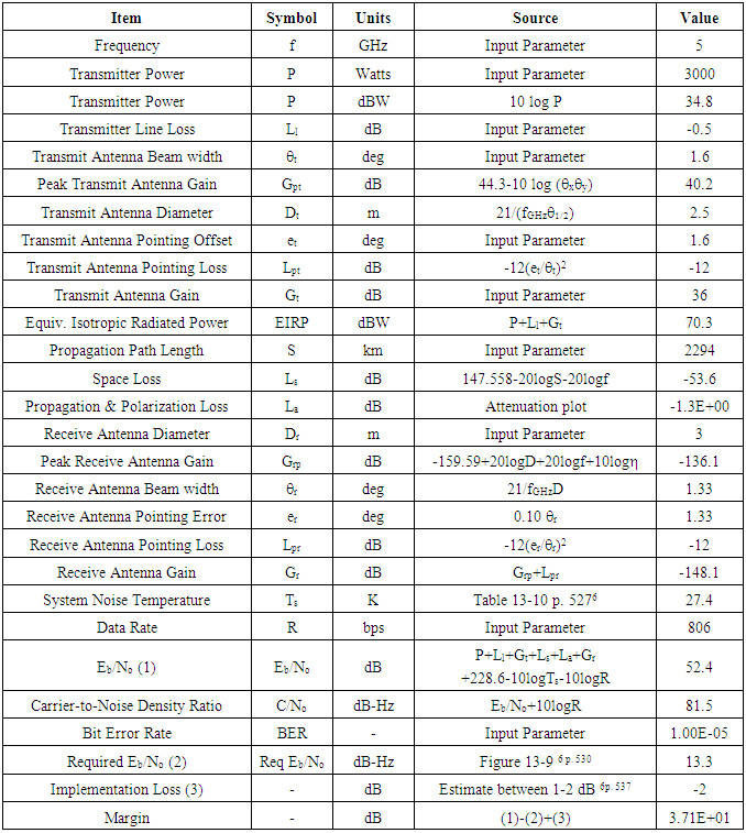
3.3. Link Analysis
- Link design describes the relationship between the transmitter power, antenna size, data rate, and propagation path length. The goal is to end up with a positive margin value. If the margin value is not positive, JSBEWS will have to iterate these parameters until positive margin is achieved. This is one of the strengths of using existing satellite radar systems as starting points. The hope is to achieve positive margin with minimal iteration. Since the link analysis is far too extensive to elaborate each calculation, the equations used and sources are cited below with the results tabulated next. Carrier frequency was selected above to be C Band at 5 GHz. This frequency is not currently a Federal Communications Commission (FCC) allocated satellite frequency. This will be a Space Law and Policy issue that must be addressed. Transmitter power is typically determined by satellite size and power limits. JSBEWS has baselined existing systems, so this yields first order estimates of design size, power and transmitter characteristics. Typical system noises are tabulated in Larson and Wertz [11] accounting for antenna noise, line loss noise, receiver noise. The beam width, gain, antenna size, and mass were selected from typical spacecraft antennas. [11]The maximum antenna offset was set equal to the beam width anticipating jamming threats anywhere in the beam width. This will drive the satellite stabilization error and station keeping accuracy. It means that the payload will gimbal a lot creating many disturbance torques which must be countered by the spacecraft attitude control system (ACS). Transmit antenna gain towards the threat emitter was calculated [11]. Space loss was also calculated [11] using the max slant range from above for the propagation path length. This provides a worst-case analysis. Propagation path loss was estimated [11] adding a loss of 0.3 dB for polarization mismatch and another 1 dB for radome loss. [11] Ground station receiver parameters are threat dependent, so they were generally estimated (e.g. antenna diameter was estimated to be identical to satellite transmit antenna diameter = 3 m). The receive antenna gain towards the satellite was calculated next using similar estimations. Theoretical vertical one-way attenuation from altitude to the top of the atmosphere was extrapolated. [11] Threat efficiency was assumed to be 1.0 (quite unrealistic, but conservative). System noise was taken from tabularized data of similar space systems. [11]
|
3.4. First Design Choice: System Scope
- There is positive margin using typical components. Next, examine some potential system design options: 1) modified version of existing radar spacecraft (e.g. SIR-C), and 2) new free-flyer satellite. It is already demonstrated SIR-C can be used since the radar range equation calculations and link analysis were based on a 3000W jammer signal. SIR-C transmits this sort of power at the same frequency we’ve baselined (C Band, 5 GHz). Assuming that it will be extremely easy to modify the modulations of SIR-C for the purpose of jamming, the remainder of this manuscript will focus on engineering development for a jammer satellite, constantly comparing the satellite effort to a modification of SIR-C. In the following paragraphs first order engineering design analysis is performed to get a better picture of what kind of effort a free-flyer new design would be. All along, modifying SIR-C will be favored as the simplest approach, but offer the analysis for the sake of completeness. It will also provide information for future development of the concept. If space-based jamming can be proven effective with a modified SIR-C flight, the armed forces might want to know what it would take to have a dedicated electronic warfare (EW) satellite.
3.5. Satellite Bus Design 1st Estimates
- I begin with the spacecraft configuration drivers [11] using statistical analysis to represent the state of current technology, yielding the first estimates of system and subsystem budget parameters. A more detailed analysis follows to verify the legitimacy of the choices and assumptions for JSBEWS. Spacecraft dry weight is driven by the total payload weight. The payload is where it all begins. So far we’ve sized the transmitter power and antenna size. The antenna mass is 29.4 kg as determined from table 13-16 [11] and the choice of a steerable parabolic 2.5 m antenna. Satellite transmitter power, mass and rf power output are plotted on curves derived from actual flight hardware relatively independent of output frequency in Larson/Wertz fig 13-15 [11]. JSBEWS will use traveling wave tube amplifiers. While heavier, they can produce higher output powers requiring lower input powers. However, traveling wave tube amplifiers require higher voltages leading to lower reliability. Future solid-state transmitters should be more capable and are envisioned to be upgraded in future designs. [11] Larson & Wertz provides empirical relationship curves for payload power versus spacecraft power. The traveling wave tube curve is roughly linear on a log-log scale allowing some complicated extrapolation, while the solid-state curves show a steep nonlinear curve for payload power on the order of JSBEWS. A linear approximation yields an input power of Pinput=1061W. Expecting more like a 100%-300% power input-to-output requirement, this is unrealistic. The extrapolation of the Larson and Wertz curves turns out to be a poor idea. Instead, let’s use the antenna dimensions to calculate a sizing ratio (another technique from Larson/Wertz). This ratio can be used with equations 9-36 through 9-41 in Larson and Wertz to determine size, weight, and power estimates.
 | (10) |
 | (11) |
3.6. Density Derived Spacecraft Volume
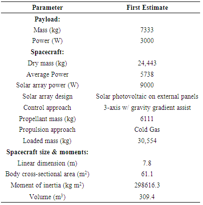
- Spacecraft dry weight is between 17% and 50% [23] of the payload weight with an average of 30%. Assuming an average 30% payload weight, a JSBEWS satellite version of the Shuttle SIR-C would weigh 24,443 kg. This is an estimate of dry weight. Satellite propellant is normally between 0-25% of the spacecraft dry weight. [23] Assuming a worst case of 25 % gives us a propellant weight of 6111 kg bringing the spacecraft total to 30,554 kg. This estimation technique is used to estimate the weight of a free-flyer satellite. A shuttle version of JSBEWS would be closer to SIR-C’s architecture (smaller, etc). Spacecraft volume must accommodate both payload and satellite subsystems, but can be initially estimated using statistical satellite densities between 20 kg/m3 and 172 kg/m3, with an average of 79 kg/m. [23] Assuming an average satellite density, JSBEWS will be 309 m3. These volume and weight estimates indicated the need to launch a free flyer satellite on the Space Shuttle or perhaps a Delta IV Heavy. Designing both versions of JSBEWS to fly on the same launch vehicle will greatly simplify the launch architecture investigation later. It will also drive a high launch cost for such large launch vehicles. The dimension, body area and moment of inertia are estimated using table 10-29 in [24] and are summarized in the table below of tabularized “1st estimates of design configuration drivers”.
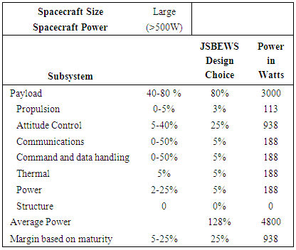
3.7. Power Budget Yields Average Power
- Solar array size may be estimated to produce 100 W/m2, so 30 m2 solar arrays will be required for JSBEWS payload. 900 m2 will be required for the whole spacecraft using SIR-C as a starting point. Solar arrays are feasible for JSBEWS, but would likely involve external panels. Solar photovoltaic arrays can produce 200-25,000 W, while solar thermal dynamic arrays can produce 1000-300,000 W. [11] Radioisotopic and nuclear power generation could produce legal or political complications. Since solar arrays are sufficient these more politically tenuous options can be avoided. Let’s take another look at electrical power by completing an estimated power budget. Earlier, we took a rough estimate of payload power, and then satellite power using Larson and Wertz equations and SIR-C as a reference. Now, it is time to define a power budget with some more estimation techniques from Larson and Wertz. [11] JSBEWS fits in the “large” subdivision based on power requirements. Accordingly, estimated power of satellite subsystems are approximated below. This is the first order design budget. Further considerations will be discussed later about these design areas and refine estimates where such is possible.
3.8. First Estimates of Design Configuration Drivers
- As you can see in Table 9 below many assumptions were made. Generally, test and evaluation communications architectures and command and data handling schemes are quite complicated. For the case of JSBEWS, the satellite will not require complicated ground control for operation. It is baselined as an autonomous jammer that will jam upon receiving threat radar emissions presumably only at certain orbital positions and altitudes. For this reason, I have assumed low percentages in those categories. The payload will require the most power. The robust attitude control architecture is assumed to be the major spacecraft component effected by the payload and is allotted a high power budget percentage above. This also allows considerations for expansion of the JSBEWS concept with more massive jammer antennas if required at higher orbital altitudes.
|
|
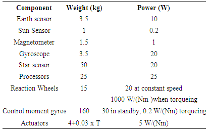
3.9. Attitude Control System (ACS) Design [11]
- The design now has a first statistical estimate of attitude control requirements. Attitude control will be very important to keep the jamming energy focused on the threat emitter, and accordingly several lines of current and future research [29]-[78] are described at the end of this manuscript. Now let’s talk in some detail about the attitude control requirements and allocate the requirements into hardware requirements. A robust attitude control architecture has been chosen to allow higher reliability to a critical wartime mission. A robust system will translate directly into higher costs, hardware, and power requirements. I favor modifying SIR-C for an initial proof-of-concept to initially avoid these high costs and requirements. The payload determines the spacecraft pointing requirements. Gravity gradient is the most simple and provides typical accuracy on the order of 5° in two axes, but is not sufficient alone for JSBEWS. The war fighting requirement would require fast spacecraft stabilization after the large antenna slews to point and jam a threat emitter. Additionally, if the antenna gimbal fails, the ACS must be responsive enough to point the entire satellite at the threat emitter. Gravity gradient stabilization schemes involve using booms and dampers for control with sun sensors, magnetometers or horizon sensors for attitude determination. Booms and dampers simply do not stabilize the spacecraft attitude quickly enough after such a large momentum input. Gravity gradient may aid three-axis stabilization architectures, if the spacecraft shape allows such a mass gradient. Three-axis stabilization will work well for JSBEWS with the Earth as the local vertical reference detectable by a horizon sensor for pitch and roll. Sun sensors or star sensors must be added to obtain a third axis reference. A course reaction control and maneuvering system must be added to damp out the large maneuvering momentum inputs and allow momentum dumping from a fine control pointing system. Reaction wheels, momentum wheels, or control moment gyros can be used for fine pointing control. This allows fine control without using a lot of fuel. A momentum wheel or thruster system (or both) for course control would allow momentum dumping from the fine control wheels. A thruster system will ultimately be required for JSBEWS. A high slewing rate (>0.5o/s) should be baselined for JSBEWS to allow maximum jamming-time of the threat emitter. For that reason, expect control moment gyros and/or two thruster force levels (station-keeping and maneuvering). The payload is going to gimbal to the local horizon nominally. Selecting such a robust and redundant attitude control system does two things: 1) allows us to quickly damp the motions of the gimbaling payload, 2) provide a fallback jammer-pointing plan. If the payload antenna fails to gimbal properly, the entire satellite can be maneuvered to put the jamming energy on the target (i.e. the slang “trons on target”) insuring successful warplane defense. The following component estimates may be summarized using all “heavy” assumptions for the satellite. Many equations provided [11] the results tabulated in Table 10.Once again, this is conservative and does not reflect the bare minimum required to accomplish the Test and Evaluation (T & E) mission, which is envisioned to be done by modifying SIR-C hardware. The summary table above is useful when considering follow-on levels of JSBEWS development, namely satellite constellation defense from surface-to-air missiles.
3.10. Free-flyer Spacecraft Design Configuration Drivers Summarized
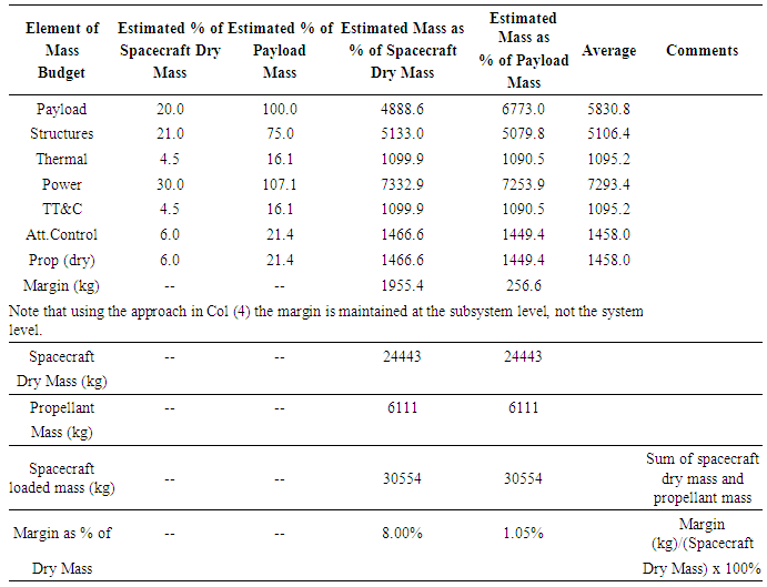
- Initial design budgets are listed in Table 11. Additional design budgets include mass, thermal, and reliability budgets. They are the pre-assigned limits for each design category to carry into subsequent phases of satellite design. For example, they provide guidance for the thermal design team by telling them how the mass of thermal control equipment they have been allotted in the overall spacecraft design. If their thermal designs exceed the pre-assigned power budget, they must perform trade studies, or renegotiate the power or mass budget with the overall spacecraft design manager.
|
3.10.1. Mass Budget
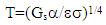
3.10.2. Thermal [66]
- The thermal subsystem of a spacecraft maintains temperature in an environment where diurnal temperature shifts are remarkable. Internal components of the spacecraft are not the only source of heat. While the temperature must be regulated as the internal components dissipate heat in a small, enclosed space, there are other drastic heat sources in space per figure 8. The sun emits thermal energy. The Earth emits thermal energy and also reflects solar energy to the spacecraft (referred to as albedo). The picture below should help easily see how heat moves in and out of the spacecraft. Thermal control may be done actively or passively typically using thermal coatings, thermal insulation, space radiators, and electrical heaters and thermostats. Cold plates are also used to mount equipment and dissipate heat. Since the incoming heat is well known, concentrate on the heat emitted from the spacecraft. Planck’s equation gives the monochromatic radiant energy from the surface of a black body. A monochromatic emissivity may be added to the numerator to get the radiant energy from a real surface.
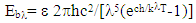 | (12) |
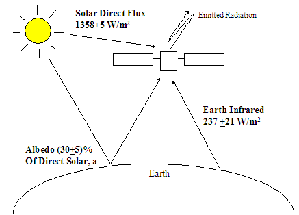 | Figure 8. Thermal environment |
 | (13) |
 | (14) |
 | (15) |
|
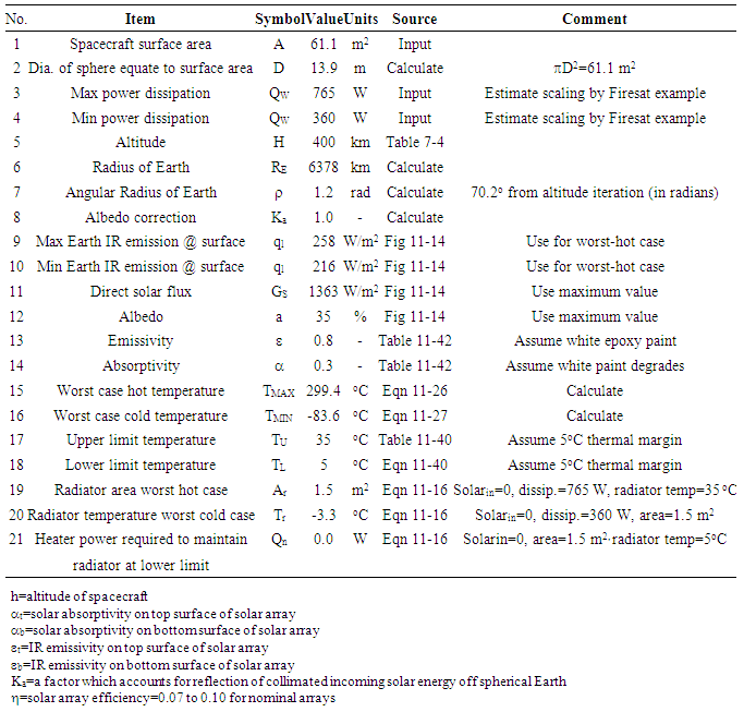
 | Figure 9. Thermal design options |
3.10.3. Satellite size and Launch Vehicles
- The satellite size cannot be so large that it equals the launch vehicle fairing size displayed in Figure 10. As you can see from the figure above, [26] the design must allow for vibration and movement within the fairing by maintaining a safe clearance. The “usable diameter” in the picture above accounts for this. It is smaller than the fairing diameter to allow movement in high vibration environments. During launch the environment is the most violent that the spacecraft will likely see in its lifetime, excluding perhaps testing. Ascent can be characterized by thermal variance between 10-35°C with heating of 188 BTU ft2/hr on the pad, and 100-150 BTU ft2/hr during ascent due to aeroheating. Accelerations of 5-7 g are common with vibrations of 0.1 g2/Hz and acoustics of 140 dB with shock values of 4000 g. [11] Considering this, remember not to get too aggressive in trying to fit the spacecraft into a smaller launch vehicle to reduce launch costs. The initial spacecraft weight indicates a need big rockets. Only two available boosters today suffice: the Space Shuttle-equivalent missions like Atlas V and Delta IV Heavy. [11] Delta IV Heavy is barely able to meet the initial estimate. This immediately leads to an expectation of lower design mass and smaller launch vehicle requirements as the design matures, since radar systems have been launched on such vehicles in the past. Regardless, a Delta IV-class vehicle or the Atlas V will likely be necessary for a free-flyer JSBEWS.
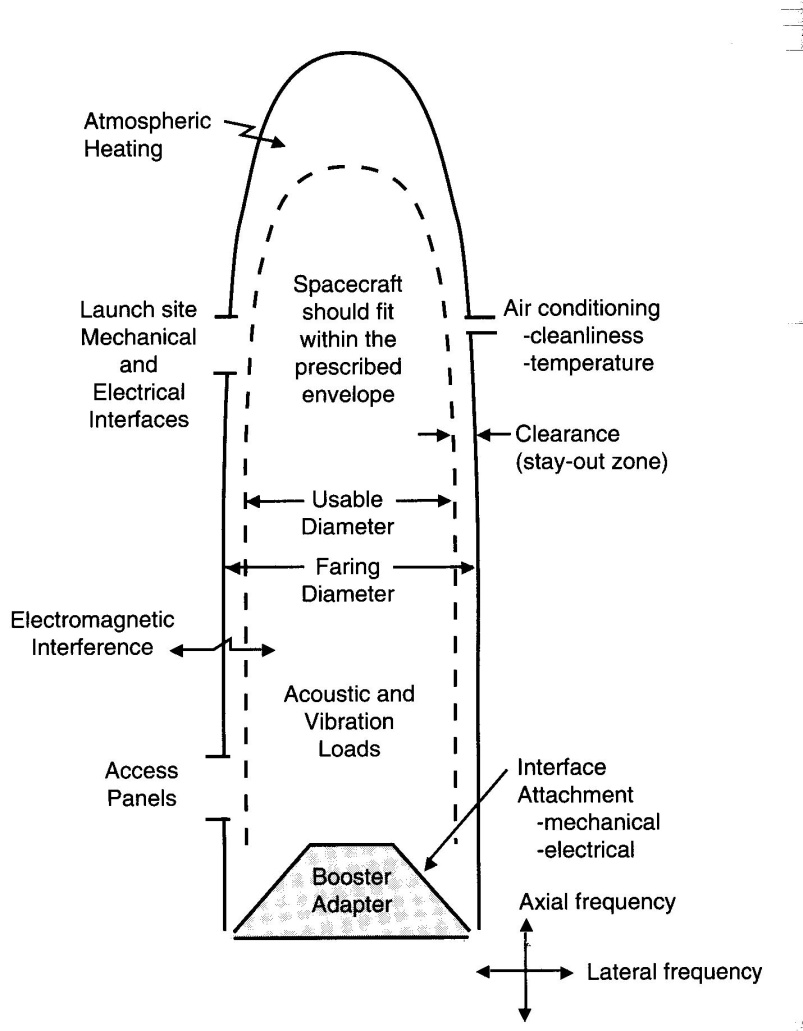 | Figure 10. Launch Vehicle fairing designs |
3.10.4. Reliability
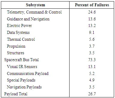
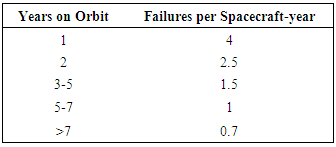
- Reliability is a subject that must be addressed from the very beginning. While this system is too immature to produce useful detailed design budgets for the free-flyer concept, it is useful to investigate the likely causes of failures to indicate where to put heavy emphasis. A shuttle version of JSBEWS (modified SIR-C) would have a nearly identical reliability budget as the original SIR-C. Accordingly, the emphasis lies in reliability of producing the modulated or unmodulated jamming signals. A systems perspective would indicate any failure effects that the new hardware or software has on other components in the system. This increases the need for a continued Failure Modes and Effects Analysis (FMEA). Benefits of FMEA at all levels are cited in [11] p. 712:At the component level to avoid high risk design decisions, such as unnecessary proximity of two conductors that can cause a catastrophic short circuit. At the subsytem level to identify single-point failure modes and the need for redundancy (fault tolerance). At all levels (including spacecraft) to aid in designing and placing mechanisms for monitoring systems, detecting errors, and reconfiguring, so the mission planner can avoid environments that can worsen unprotected failure modes. A histogram is useful to indicate where failures typically occur in space missions. It provides a good sense of the state of technology today. For example, if most failures are caused by propulsion systems, leading to an emphasis on propulsion. As it turns out, propulsion is a very mature technology today and most failures are not caused by propulsion systems. In general, 73% percent of failures are attributed to the spacecraft bus as opposed to the payload. The failures are listed by percentages in Table 14.
|
|
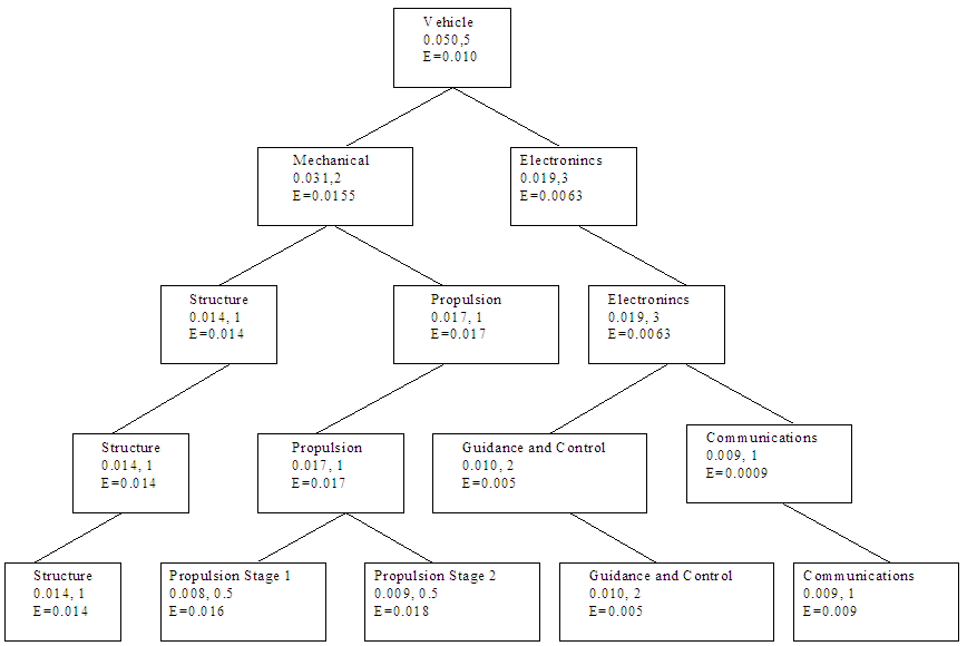 | Figure 11. Probability tree |
3.11. Ground Operations Architecture & Launch Services
- Figure 12 was taken from RADARSAT [22] for synthetic aperture radar (SAR) imaging. It is useful as a reference when talking about the satellite flying over ground points depicted by the patches of shaded areas on the lower part of the figure. The satellite path in the sky remains a fixed trajectory. The area on the ground that can be jammed however is not simply a straight line under the trajectory. The jammer antenna can gimbal to point jamming energy at a pre-selected point on the ground that is within its viewing limits. So, pick points along the trajectory to place threat emitters. Another option is to pick the orbit such that it flies over a known threat location. By choosing the intended emitter to be an aircraft jamming scoring site (explained next), an evaluation of the jamming effectiveness is immediate. The spacecraft jamming evaluation can be performed in the same manner as jammer aircraft scoring. The scores would indicate whether or not the space system could jam threat emitters as effectively as aircraft jamming platforms. This minimizes onboard processing requirements and eliminates the need to design and buy a dedicated ground data processing network. Satellite ground control will be performed by the Air Force Satellite Control Network (AFSCN). Anticipate ground control to be performed by the Air Force Space Command.Similarly, expect launch to be performed by the US Air Force for a free flyer satellite. The “NASA” version of JSBEWS can use Shuttle military launch credits managed by the DoD Space Test Program (STP) office at Johnson Space Center. These credits allow the military to fly for free in exchange for the military financial support given to the Shuttle during its initial development. The STP also funds integration of military experiments. STP funding can be obtained to modify the SIR-C radar emissions by presenting this system design to the DoD Space Experiments Review Board (SERB). When STP support is achieved JSBEWS will not require any newly developed launch or operations architectures.
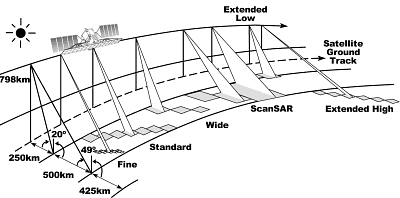 | Figure 12. Target acquisition, tracking, and spacecraft fine pointing |
3.12. Threat Emitters & Evaluating the Jamming [22]
- Electronic scoring against simulated threat emitters will be done exactly like it is done for aircraft jammers. Aircraft fly over sites with simulated threat radars. These sites have well known latitude and longitude coordinates. A planned satellite flight path over any of these sites will allow s jamming to be scored in the same manner that it scored for aircraft jammers. This eliminates the ground station data processing requirement and also normalizes the data for comparison to other aircraft jamming options. Many threat radar simulators systems exist throughout the world. The systems discussed next are claimed to be used for air crew training in Jane’s Radar and Electronic Warfare Systems [78]. The AN/MST-TA(V) Mini-MUTES Electronic Warfare training system allows aircrews to experience dense multiple radar threats duplicating an enemy Integrated Air Defense (IADS). Each of 1-5 Remote Emitter Units (REUs) can: Ÿ acquire automatically and track a co-operative aircraft and direct emitter signals Ÿ permit multiple identification friend-or-foe (IFF) acquisition and tracking modes, and pointing and slaving modesŸ record electronic countermeasures and aircrew response to the simulated radar emissions with corresponding flight path dataŸ process noise jamming detection, range gate pull off detection, velocity gate pull off detection, and amplitude modulation detectionŸ send status, pointing and tracking data, ECM receiver data, and fault and warning messages.The AN/MST-T1A MUTES multiple threat emitter system is capable of simulating threats over a specified frequency range with accuracy sufficient to activate radar warning receivers and electronic countermeasures systems. The system can simulate, for example, surface-to-air missile engagement radar, together with appropriate missile guidance signals. MUTES can simulate a wide variety of radars including height finding, ground control intercept, aircraft intercept, surface-to-air missile acquisition, tracking and missile guidance, and anti-aircraft artillery radars.Other systems include the AN/MSQ-T13 and the AN/MSQ-T43. They include pulse repetition frequency generators, multi-beam acquisition receivers, transmitters and associated hardware. These systems are capable of simulating missile launching and/or anti-aircraft artillery threat radar systems for aircrew training. Many other systems are listed in Jane’s. I mention only a few here, but the list goes on. Any of these systems are sufficient to score JAMSAT electronic interference jamming. The score would by default be normalized to any aircraft jammer that uses the system to score ECM training.
|
3.13. Manned Versus Unmanned Missions
- Aircraft jammers have a man-in-the-loop called an Electronic Warfare Officer (EWO). This option remains available for modified SIR-C hardware. A free-flyer satellite can also have an active EWO conducting electronic combat through a ground station uplinked to the spacecraft jammers and receivers. A EWO onboard the Shuttle provides real-time human intervention to critical combat situations and is definitely recommended for the Shuttle modified SIR-C concept. Plans can be in place to quickly change the manifest of upcoming shuttle missions to include JSBEWS and an EWO. This gives the United States a relatively responsive capability to increase short term electronic warfare capabilities until more assets can be positioned in theater for protracted confrontations.
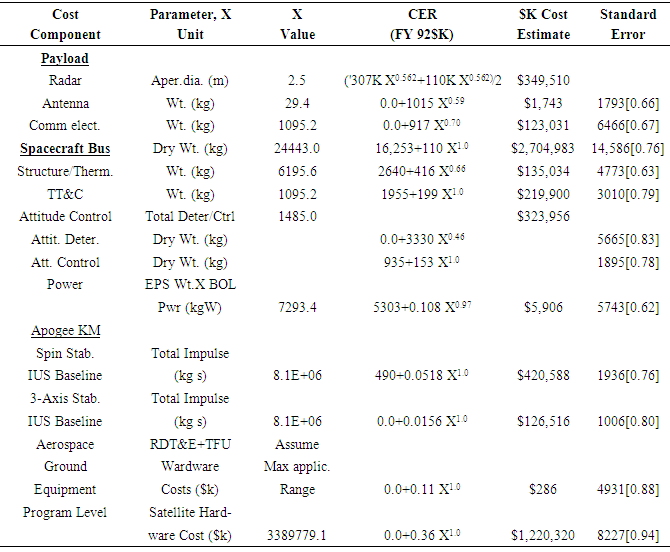
3.14. Costs
- As mentioned previously, the JSBEWS SIR-C modification design will request STP funding through the DoD SERB. This will cover modification of the SIR-C radar emissions. STP will also provide a free launch and one year of satellite ground control. Essentially, the SIR-C version of JSBEWS would not require any funding other than overhead for the project management (also proposed to be handled by the Air Force laboratories). The free flyer satellite however is an entirely different issue. Key satellite parameters directly relate to costs and are used to estimate the costs of future satellite ventures. Using the same satellite database as used in the engineering design, the following cost estimations have been made.The immense magnitude of a free-flyer satellite effort is obvious. A constellation of electronic warfare satellites is an effort on the order of Global Positioning System (GPS) or Defense Support Program (DSP). The good news is that it seems that costs may be coming down in the future. The upcoming upgraded RADARSAT mission is estimated to cost $305 million vs. more than $600 million for RADARSAT-1. If this is true then reference-6 estimation techniques must be updated to reflect this. Regardless, the cost is enormous. It is for this reason that the military cannot afford to proceed without a demonstration that the concept is sound. Satellite based electronic combat must first be proven with a small scale effort like an Electronic Warfare Officer using modified SIR-C hardware to jam ground training sites. After such a demonstration, decisions regarding free-flyer satellites can be made safely leaving the Shuttle/SIR-C concept available for short-term electronic combat assistance.
3.15. Follow-on research
- Figure 12 revealed a key operation feature of jamming from space, namely target acquisition, tracking and spacecraft fine pointing. Section 3.1 illustrated that small pointing errors on-orbit lead to large errors tracking the target threat emitter. At least two main areas of research were investigated: 1) maximizing spacecraft rotational actuator torques, and 2) adaptive system identification and control to account for time-varying factors like fuel use and also account for disturbances and potential battle damage.
3.15.1. Maximizing Spacecraft Rotational Actuator Torques
- Torque generation is to be performed by momentum exchange devices, since using expendable propellant drastically limits on-orbit mission life (limited by the amount of propellant onboard). Control moment gyroscopes are the most effective momentum exchange device [11], but their steering has mathematical singularities that can result in complete loss of attitude control, especially during aggressive maneuvering [30]. Despite singularity issues, CMG research began in 1960s for large satellites like SKYLAB. Computers of the time could not perform matrix inversion real time. Simple systems that did not require matrix inversion were an obvious choice. Otherwise algorithmically simple approximations must have been available for the system chosen. Singularity avoidance was researched a lot in the 1970s and 1980s [31]-[35].Singularity avoidance was typically done using a gradient method [34]-[35]. These gradient methods are not as effective for Single Gimbaled CMGs (SGCMGs) as for Double Gimbaled CMGs (DGCMGs). Margulies was first to formulate a theory of singularity and control [36] including the geometric theory of singular surfaces, generalized solution of the output equation, null motion, and the possibility of singularity avoidance for general SGCMG systems. Also in 1978 Russian researched Tokar published singularity surface shape description, size of workspace, and considerations of gimbal limits [38]. Kurokawa identified that a system such as a pyramid type CMG system will contain an impassable singular surface and concluded systems with no less than 6 units provide adequate workspace free of impassable singular surfaces [39]. Thus MIR was designed for 6 SGCMG operations. Continued research aimed at improving results with less than 6 CMGs emphasized a 4 CMG pyramid. Many resulted in gradient methods that regard passability as a local problem that proved problematic [37]-[39]. Global optimization was also attempted but proved problematic in computer simulations [41]-[42]. Difficulties in global steering were also revealed in Bauer [43]. NASA [44] compared six different independently developed steering laws for pyramid type single gimbaled CMG systems. The study concluded that that exact inverse calculation was necessary. Other researched addressed the inverted matrix itself adding components that make the matrix robust to inversion singularity [44]-[46] as extensions of the approach to minimize the error in generalized inverse Jacobian calculation [49]. Path Planning is another approach used to attempt to avoid singularities that can also achieve optimization if you have knowledge of the command sequence in the near future [46]-[52]. Another method used to avoid singularities is to use null motion to first reorient the CMGs to desired gimbal positions that are not near singular configurations [53]. Despite the massive amount of research done on CMGs, precision control w/ CMGs is still an unsolved problem [50]-[54] and is the focus of considerable recent research. Very recent research [55]-[61] has provided several good techniques, and research in this area continues.
3.15.2. Adaptive System Identification and Control
- Adaptive control with online system identification [62]-[65] has proven very effective for controlling spacecraft pointing very accurately, and this initial research was merged with “physics-based” control [66]-[71] with increasing effectiveness. Mostly recently [72]-[79] individual system components (down to the controller circuits) have been adaptively controlled with online system identification to further amplifying the physics-based nonlinear adaptive control methods for spacecraft fine pointing.
3.16. Future Efforts
- Immediately, the component-based expansion of adaptive techniques will be develop for additional spacecraft components (additional actuators and also sensors). Furthermore, recent ventures to increase critical thinking in the American nuclear enterprise [80], [81] following the recent publication of the nuclear posture review [82], [83] provides opportunities to include these technical areas in response to the trending national security challenges [84], [85].
4. Discussion and Conclusions
- This project verified that a joint space-based electronic warfare satellite (J-SBEWS) is quite feasible and useful: technically, legally, and politically. The applicable treaties and political topics necessary to declare J-SBEWS a viable option for the future were elaborated. Technical feasibility was demonstrated using calculations and simulations of the radar equation and link design which produced ranges for key system parameters, which were subsequently used towards a first-of-its kind space mission design. Astrodynamics reveals that a low-earth orbiting altitudes of 100-400 kilometers produces jamming effects on the target emitter for 4.8-10.2 minutes respectively producing jammer energy received by the targeted radar of -23.9 to -102.9 decibel-watts respectively. These key design features are used to establish a link-budget that reveals mission margin. First-order engineering design relies heavily on empirical engineering relationships derived from actual flight hardware. Spacecraft key design budgets were calculated next revealing the requirement for a large spacecraft (~7333kg, 7.8m X 61.1m2) and large launch vehicle (Atlas V class). Budgets are also found for key satellite subsystems: payload, structures, thermal, power, TT&C, attitude control, and propellant. Reliability calculations and cost estimated were discussed, and normalized evaluation of jamming effectiveness is recommended. Lastly, key technology challenges of target acquisition, tracking, and spacecraft fine pointing are discussed, and current research efforts are highlighted inspiring future directions for technical innovations to enhance the design.