Branko Mišković
Independent, Novi Sad, Serbia
Correspondence to: Branko Mišković, Independent, Novi Sad, Serbia.
| Email: |  |
Copyright © 2015 Scientific & Academic Publishing. All Rights Reserved.
Abstract
Electrodynamics of moving bodies, including the bases of the classical EM theory, without the considerations related with its practical application, is here presented. Initial symmetry of the two EM fields is gradually overcome and substituted by the trinity of the static, kinetic and dynamic relations. The two alternative basic sets, algebraic equations and central laws, complementary with the standard differential equations, are finally elaborated. This is the educational exposition in the form of a sequence of successive lessons, on the middle university level. A number of the advances in the contents and form gave the completely new whole. Though innovative and extended, it is more transparent and convincing than the standard presentations of EM theory. Some fundamental theoretical problems, so far inconsistently treated by the incomplete standard theory, are resolved and/or reinterpreted.
Keywords:
Electrodynamics, Moving bodies, EM theory, Standard presentation
Cite this paper: Branko Mišković, Fundamentals of Electrodynamics, International Journal of Electromagnetics and Applications, Vol. 5 No. 1, 2015, pp. 22-65. doi: 10.5923/j.ijea.20150501.04.
1. Introduction
EM theory initially started by Coulomb’s laws describing the static interactions of magnetic poles or electric charges. The analogous Ampere’s problem, of the kinetic interaction between two moving charges or elementary electric currents, had not been formulated in its most general form. Further development thus continued on the electric circuits, mainly observed at rest. It is finally crowned by the four Maxwell’s equations, as the differential basic set. With experimental investigation of moving media, H. Hertz extended two of these equations, by some algebraic terms – into the hybrid form. However, he failed both, to complete the new set and explain his own experimental results by it.On the other hand, H. A. Lorentz considered convective electric currents, and obtained respectable theoretical results. Despite ellipsoidal field deformation, he predicted the even distribution of EM forces about the spherical surface of a moving particle. With some empirical helps, he formulated the mass function against the motion. However, he did not determine the reference frame for the speed determination. In this sense, various experiments gave unexpected, as if – mutually disparate – results. In this situation, A. Einstein proposed SRT, as a speculative interpretation. The collision with the technical practice is avoided by the parallel and independent presentations and teachings.The classical theory is also founded in a few approaches. Apart from the static, kinetic central law is avoided due to its incomplete form. Both these laws are finally substituted by two pairs of differential equations. In addition, at least one algebraic relation is used. In the attempt of its further elaboration, it was disturbed by the relativistic correction. With two basic set, respective interpretations of the force actions were understood: directly at a distance – at central laws, or by the successive force transfer – at the differential equations. In a similar form, this dualism is also transferred into the modern physics: SRT is nearer to the former, and quantum theory – to latter views.We present EM theory in the three levels, represented by EM carriers, their fields and potentials. Central laws thus constitute its fundament, differential equations – its walls, and algebraic – its floors. With respect to the incomplete fundament, the walls were built by intuition and experience. Further trying to mount the floors, SRT was introduced. Its provocative opinions are the additional motive of this our elaboration. Oriented by the walls, the floors are somehow mounted. The final completion of the fundament gives the solid basis for the higher aspects of this scientific building. Their direct mutual relation demands some reinterpretation of the former principal scientific views.The classical and modern concepts of the particles, their fields and interactions are overcome. Instead of the source or carrier of its field, a particle is treated as the field center. Instead of the field macro-sum, the multiple rigid, stably oriented elementary fields are understood. In the zero sum of such two opposite fields, the moving fields manifest their own kinetic effects, independently of the opposite resting fields. In accord with the algebraic set, the fields interact directly, in each point of the space – separately. Maxwell’s successive force transfer was disparate even with his own equations, not taking into account any time for the force transfer between interacting particles.A principal misunderstanding from the technical practice and its formal interpretation should be also overcome. By the known medium stratification, the total EM fields (D,B) are resolved into their vacuum (E,H) and material (P,M) components. At the homogeneous and isotropic present media, respective two components are collinear, forming in common the total fields, in the same forms. The irregular media deform the components and their sums, with the final tensor relations of the primary and total fields. Imposed by the practice, this complication imports some confusion in the basic EM theory. Instead, we understand the constitutive equations relating the proportional final components of the total fields, by the two scalar constants.The Newtonian reaction on scientific arbitrariness is also taken into account. Instead of unfounded assumptions in the particular situations, all available or at least more relevant possibilities are considered. Being obtained by temporary use of the assumed magnetic poles, the results are finally restricted to the empirical facts. Instead of the relativistic or non-relativistic approaches, as the thesis and anti-thesis, some their synthesis is finally obtained, taking into account the valid details and convincing results from each of them. The former incomplete field transformations are extended, thus removing their asymmetry. At least in principle, the orientation in space and time is resolved.The mentioned series of relatively new views and results represents the sufficient basis for systematic and methodical exposition of EM theory. A few algebraic are added to the standard differential equations. The complementarity of the two basic sets and their applications is demonstrated. All these procedures demand some rearrangement of the formal aspects of the theory. The obsolete terms are substituted by more adequate ones, pointing to logical classifications of the quantities and their relations. The majority of the former symbols is kept and classified in accord with the Maxwell’s convention: discrete quantities are denoted by lower cases, and physical fields – by respective capitals.
2. Mathematical Bases
The brief cross-section through mathematical aspects of field theory, apart from their transparent presentation and repetition, explains the adopted symbols used in the theory. The logic of successive introduction of the basic notions is presented, but their derivations are ceded to the readers, as the exercises. Their essences are clearer in the applications. This overview avoids the repetition of the same procedures during following exposition of the theory.
2.1. Introduction
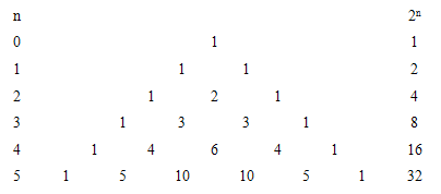
We now explain some formal conventions here adopted, not usually used in presentations of EM theory. Owing to transparency of the equations and formal procedures, with distinction of similar physical quantities and mathematical operators, the unique symbol ∂ is used: without index – at a differential, but derivative also includes the variable index (∂x = ∂/∂x). The artificial distinction of the usual and partial derivatives is thus overcome in advance.The set of n independent dimensions forms the nD-space, and its subsets represent all the kD-subspaces (k ≤ n). The numbers of kD-subspaces just accord to respective binomial factors, presented in the following table. Their sums finally give 2n subspaces of each nD-space. Its convincing logic is explained in the continuation of the text.Table 1. Binomial factors
 |
| |
|
The addition of each new axis does not disturb the former subspaces, forming with them the same numbers of higher spaces. Therefore, each new row of the binomial factors is obtained by the addition of the successive factors from the former row. The ascending column of units represents the points, as 0D-subspaces of each the space. It is successively followed by the axes, planes, etc; up to the index k reaches the value n, in each of the next rows.Unlike arbitrary orientation of the spatial axes in 3D, the direction of temporal axis in 4D spaces is determined by the cosmic expansion. Oriented in this direction, the fourth axis is preferential with respect to the three spatial axes, thus representing the longitudinal axis. The three longitudinal planes (xt, yt & zt) cut each other through the temporal axis, and with xyz subspace through three its axes. The transverse planes (xy, yz & zx) belong to 3D space xyz. Amongst four 3D subspaces, only this one is manifest.A determined quantity belongs to each of the n1 sets of the subspaces in nD space, via respective multi-vectors and forms of the motion. The scalar quantities thus accord to the points, vectors – to axes, bi-vectors – to planes, and the pseudo-scalar, anti-polar with respect to redirection of one its axis – to nD space itself. The multi-vectors are treated by respective tensors: scalar – by a number or scalar field, vector – by a sequence of n numbers, bi-vector – by the matrix n2, tri-vector – by the cube n3, etc.Though inaccessible directly by the sensory perception, physical relations from nD space can be at least estimated by generalization of the geometric relations from 3D space. A quantity from the higher space is also manifest in 3D, as respective projection into the less dimensionality, along the number of axes just concerned by this projection. This possibility provides some empirical facts for their physical interpretation. In the special case of EM quantities, being projected from 4D – into 3D spaces, the projection used in the considerations concerns temporal axis. The above table shows that – by such the projection – 4D scalar and pseudo-scalar disappear. The tree components of 4D vector keep their own status, but fourth one turns into a bipolar scalar. Of the six bi-vector components, transverse three keep the same their former statuses, but longitudinal three turn into respective polar vector. Of the four tri-vector components, the three turn into 3D bi-vector, and fourth one – into 3D scalar. The fourteen projections from 4D thus overlap in the eight subspaces of 3D spaces. Apart from the 3D scalar and tri-vector, by the three vector and bi-vector components overlap in the pairs. The identification of 4D quantities also relies on their phenomenal features and the established mathematical relations.The projection from 3D into a plane, with overlapping images, is used in descriptive geometry. Their separation and interpretation demands a considerable imagination. On the technical drawings this is avoided by projections into the three separate sheets. In this sense, the images from 4D can be presented in four 3D spaces or six planes. In both cases, the media are dislocated in 3D. At the treatment of some symmetric phenomena, the numbers of the distinct projections are considerably reduced. This is the common convenience in EM and quantum theories.
2.2. Vector Products
Two field pairs are introduced in EM theory: rational (D,H) and force fields (E,B). In tensor calculus the former pair is treated as contra-variant, and latter one as covariant vectors. Concerning the primary sense of the pair (E,H), and secondary – of (D,B), respective fields are mutually related by the mixed tensors. However, if the former fields were understood as the components of the final fields, they are simply related by the scalar constants. The distinction of the two vector types is thus overcome.We present the elements of the simplified tensor calculus, convenient for introduction of the differential operators and derivation of the needed forms used in elaboration of EM theory. At first, we introduce the dyad of two vectors in nD space, as the full set of the products of each components of one, by all components of the other vector. Arranged into a square matrix, as the dyad terms, these products in common represent the two-dimensional matrix: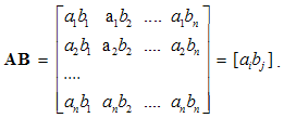 | (2.1) |
With n rows and n columns, the dyad contains n2 terms. By commutation of the two vector factors, the symmetric terms, aibj & ajbi, exchange their indexes and places in the matrix. As if, the matrix is thus rotated about descending diagonal. In other words, the dyad is transposed.By definition, the sum of diagonal terms of the dyad of two vectors forms their scalar (dot) product: | (2.2) |
As the 0D-tensor, this is a scalar, as the projection of one, on the direction of the other factor. This interpretation may be also used at the dot product of a vector and tensor.The difference of a dyad and its transposition, as if being complementary to the dot product, gives the bi-vector, anti- symmetric 2D-tensor with zero diagonal terms: 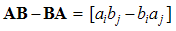 | (2.3) |
Unlike two starting vectors, expressing axial translations, the bi-vector expresses the rotation in a plane. The opposite symmetric terms concern the same coordinate planes, or the axes being perpendicular to them. With respect to the same numbers of the planes and axes in 3D space, each such bi-vector may be associated with the orthogonal axial vector, directed along the axis of rotation. In this way, the cross- product vector operation is introduced. By this its definition, this product is restricted to 3D space: 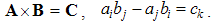 | (2.4) |
It equals to the surface of the parallelogram determined by the two factors. As the axial vector, it is perpendicular to the surface. Such a product of two collinear vectors, and also of a vector by itself, annuls. Unlike the commutative dot product, this one is anti-commutative. With respect to (4), this fact just means: B × A = − C.By means of the defined two products, the two following vector identities can be confirmed: | (2.5) |
 | (2.6) |
The former is mixed, and latter – double cross-product of three vectors. The former represents the volume of the cub determined by the three factors. A repetition of one factor in this product would thus annul this volume.
2.3. Spatial Derivatives
The three spatial derivatives (div, curl and grad) can be suggestively introduced as respective products of the given vector field by the symbolic vector nabla (∇): | (2.7) |
 | (2.8) |
 | (2.9) |
Here the sum ∑ ∂iii = ∇ represents the vector. In 3D space, as the domain of these operations, the index (i) takes the values 1, 2 & 3, with the unit vectors ii. By these definitions, divergence is the dot product, curl – cross product, with the gradient as the symbolic dyad itself. Apart from the vectors, some of these derivatives can be applied to the scalars and tensors. In this sense, gradient of a scalar is vector, as well as the divergence of a dyad of two vectors.There are now the spatial derivatives of a few elementary functions. Thus, the divergence of radius-vector equals to the number of the axes (n). Therefore, in 3D space ∇·r = 3, but in a plane ∇·r = 2. The application and reduction of the equality (17) directly give: ∇ × v = 2ω, where ω = r × v is angular, and v – peripheral speed of rotation.In graphical sense, divergence is presented by beginnings & terminals of the field lines. Unlike its etymology, it does not concern the moving away of the field lines. However, these both aspects constitute the longitudinal field gradient. On the other hand, the field curl includes the line curvature and transverse field gradient. In the case of unidirectional fields only, their divergences equal to the longitudinal, and curls – to the transverse field gradients.
2.4. Complex Operations
Dot product of one, by gradient of another vector – as the tensor, consists of n numbers, and so is a vector: | (2.10) |
The latter order avoids the gradient, thus restricting the procedure to the set of vectors. The two kinetic derivatives, relative and convective, are in this form: | (2.11) |
Here v is the object speed, and V – that of the moving field A. The relative derivative is proportional to the object speed and the resting field gradient, but convective one is opposite to the moving field gradient at a resting point. The last equality relates these two – with respective temporal derivative, expressing the field variations.By means of above differential operations, the following forms can be routinely confirmed. As the first, there is the divergence of the dyad of two vectors: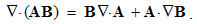 | (2.12) |
In general, this operation is not commutative (13), but in the case of a scalar factor (14), it is invariant: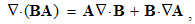 | (2.13) |
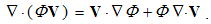 | (2.14) |
The former term of (14) is convective variation of the scalar Φ, and latter – its dilatation by speed V.There follow div & curl of a cross product: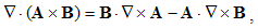 | (2.15) |
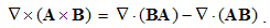 | (2.16) |
The divergence is the difference of dot product of one, by curl of the other vector. Curl is the divergence difference of the dyad and its transposition. By substitution of (12) & (13), (16) obtains the four terms: | (2.17) |
Gradient of a dot product also contains the four terms: | (2.18) |
There are also a few second order operations, e.g.: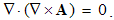 | (2.19) |
With respect to the repeated factor, the mixed product annuls. A vortical field has no its sources. Curl cannot be applied to divergence of a vector, as the scalar.The divergence of a gradient gives Laplace’s operator: | (2.20) |
If not predetermined by parantheses, the three operations have the priority in the formal procedures.
2.5. Summary
All these mathematical operations stress their imaginative essences. Instead of the formal application of the obtained results, their active derivation will help the insight into their real physical essences. The formation of respective images would be also important, at least in 3D space, with gradual generalization to the new axes. Though presented formal relations are already well-known, they have not been so far fully applied to the final elaboration of EM theory. Some advancement in this sense, made in the following exposition, is probably not completely exhausted.
3. EM Interactions
Two types of EM forces are presented: static – of the similar (E or M), and kinetic – of dissimilar (E & M) poles or charges. By means of the distributed fields, the unilateral force actions – of the field carriers upon their objects – are thus observed. The static forces act between similar poles, irrespective of their motion, and kinetic ones – between moving carriers and dissimilar present objects, or vice versa. Some symmetry of EM phenomena is pointed at.
3.1. Introduction
Similarly to the classical mechanics, the development of electrodynamics started by its central laws, describing the forces between EM poles at rest or in motion. Owing to the objective limitations of respective empirical investigation and technical practice, the theoretical development was a little obstructed. Unlike the static interaction of two electric charges, formulated and empirically tested, the kinetic force between elementary currents has not been so far formulated in the most general form. The observations of elementary particles and respective delicate measuring are realized on the bases of the incomplete EM theory. The sufficient quantities are obtained in electric circuits. Line currents, from the primary circuits, noticeably affect secondary circuits and measuring instruments. The clumsy integral laws, operating by the distributed quantities and their temporal variations, are formulated on this basis. By a convenient mathematical generalization, Maxwell turned these laws into the new basic set of the – more operative – differential equations. On the other hand, the implicit form of Maxwell’s equations was the main obstacle for their further affirmation. This disadvantage is overcome by the empirical verification of EM wave existence, just predicted in advance by these equations.Relating the measurable physical quantities, Maxwell’s equations are applicable in the practice. Even their complex resolution, as the operative disadvantage – merely surpassed by the computers, did not hinder the technical development. However, these equations are not convenient at the moving bodies. The quantities measured by the instruments resting near electric circuits do not speak sufficiently about the longitudinal field effects. The electrodynamics of moving bodies was initiated by H. Hertz & H. A. Lorentz, and then continued by A. Einstein, but some quandaries further remain. With other lacks and inconsistencies of the classical and modern physics, these quandaries were the main motive for this our elaboration of EM theory.
3.2. Basic Notions
Owing to vague essence of EM phenomena, respective theory is founded according to the effects caused by them in human sensory perception. In the aim of some interpretation of physical processes, necessary initial formal concepts are introduced, as the electric and magnetic poles or charges are, partaking in the observed interactions. The term pole is more convenient at central forces, and charge – in the field theory. The attractive and repulsive forces are explained by their division into two classes: positive and negative ones. Namely, the equipolar charges mutually repel, and opposite ones attract each other. This is the only empirical way for their mutual comparison and distinction.Apart from radial static forces, dependent on the distance of two poles, the additional forces depend on their motion. The two moving poles, as the convection currents, interact by transverse kinetic forces, in the function of the speed product, irrespective of the mentioned static forces. Some variation of an electric pole motion affects all the present poles, including this one itself, by the longitudinal dynamic forces, in the function of the acceleration. Affecting all the present poles, the static and dynamic forces in common are expressed by unique electric field, of the same direction. By the cross-product, kinetic forces are related with magnetic field, transverse to the force and motion.Two opposite electric poles connected at a distance form respective dipole. Their separate fields are added as the two vectors at each point. As such, they affect the other poles and dipoles. Some rotation of electric dipole around a pole forms the circular current and magnetic dipole coaxial with rotation. Unlike two electric poles, constituting their dipole, the magnetic poles cannot be separated from their dipole. However, the two dipoles similarly behave in respective fields. This symmetry is supported by formal similarities of the basic equations. In spite of the essential distinction, EM theory is lead astray by these symmetries.
3.3. Static Interactions
The conditional consideration of fictive magnetic poles enables parallel foundation of electric and magnetic theories. Respective Coulomb’s laws express the static interactions of electric or magnetic poles, at a mutual distance: r = rro. Unlike the non-polar mass, both EM charges are bipolar, with the wider analogy of the two laws: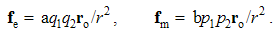 | (3.1) |
Here qi are the assumed electric, and pi – rather fictional magnetic poles. Unlike the ever attractive gravitation, EM forces may be also repulsive, depending on the parity of the interacting poles. Mutual exclusivity of the two static forces (1) points to the two distinct pole types.Apart from the medium influence, the constants (a & b) mutually relate quantities and units. The force equivalence gives the following dimensional equalities: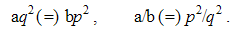 | (3.2) |
The two constants observed at vacuum reduce into their factors (ao & bo) which mutually relate and harmonize the quantities and units. Finding EM phenomena as mutually independent, Gauss arbitrarily adopted the two unit factors. In spite of the exclusive forces, the dimensional equality of the two EM charges was thus postulated.This is an additional symmetry of electric and magnetic phenomena. The ratio of the two constants is determined: a/b = c2, where c is the speed of light propagation at the present medium. The dimensional ratio of the two charges is thus also determined: p/q (=) c. With respect to this ratio, Gaussian conventions (in the rational form) are the bases for the modern natural quantities and units.The two empirical bases of electric and magnetic poles are transferred to their static relations. The latter of them is introduced by formal symmetry with the former, already empirically established. According to this relation, P. Dirac assumed the existence of free magnetic poles. Not only that such the poles have not been noticed, but the full symmetry would mean the identity or mutual independence of the two EM phenomena. Both of these consequences disaccord with experience, and the noticed phenomenal distinction must be accepted as the fundamental EM asymmetry.The static central laws (1) speak nothing about the force transfer, but understand the direct interactions of the poles, at a distance. The two EM fields causally relate the causes and effects. The two laws are resolved into the actions and distributions of static fields, as the assumed intermediate vector quantities distributed in the medium: | (3.3) |
 | (3.4) |
The left equations define external fields, via the forces acting on the present objects (2), and right ones express the central field distribution around the carriers (1).The elimination of the objects affected by central fields gives the central laws (1). As if the carriers act by their fields on the distant objects, directly at their locations. At least for the resting poles, the time needed for the force transfer is irrelevant, and so their instant action at a distance may be understood. With respect to the force symmetry, the carriers and objects may exchange their two roles, and the unilateral consideration does not disturb their equivalence. The above causal logic does neither, disturb the symmetry nor prejudice a manner of the force transfer.The two static laws treat the interactions in the pairs of similar poles. In the case of more such poles, two opposite ones may be coupled into respective dipoles: p = ql and/or m = pl. Here l is the small vector of the mutual position of the positive and negative poles. The laws of force actions (3,4-a) determine the torques and forces by which the two fields (E&B) affect their respective dipoles: | (3.5) |
 | (3.6) |
The torques turn the dipoles into the field directions, but the forces draw them into the stronger fields. These actions result from separate forces affecting each pole. The forms (5,6-b) applied to the central fields (3,4-b) give the forces declining by the third power of the distance. In general, the force between two multi-poles declines by the power equal to the full pole number. The distant interactions of neutral bodies are thus practically annulled, having the noticeable values only in their very close contact. The relations (6) are obtained from (4a) and included into (1b) somehow confirm this law. If free magnetic poles were existent, they would interact according to this law. Though such poles do not exist, the application of (4a) to respective dipoles gives the valid, empirically confirmable results. In this way, the starting asymmetry of the two EM phenomena, expressed in possible freedom of electric and indispensable connection of magnetic poles, is temporarily bypassed. In fact, the following considerations also call in question a real existence of the assumed electric poles.
3.4. Kinetic Interactions
The motion of EM charges, with respect to their material surroundings, form respective elementary currents: electric j = qv, or magnetic k = pu, where v & u are respective two applied speeds. At least electric current can be obtained as conduction or convection of free electricity: | (3.7) |
The former concerns a small segment (l) of line current (I), and tatter – the motion of a free charge (q). At the small values q & l, their linear ratio is understood: q/l = ∂q/∂l, and so q∂l = l∂q. Their equivalence is thus affirmed. There is known from the experience that each EM current produces the dissimilar field in its surroundings: electric current – magnetic field, and vice versa. This reciprocity enables the mutual kinetic interactions, between a moving charge and dissimilar field, expressed by the actions and distributions of respective kinetic fields: | (3.8) |
 | (3.9) |
The left equations define the two fields kinetically – by their actions upon dissimilar currents, and right determine the field distributions around such currents. The upper pair gives magnetic – in the function of electric quantities, and lower all the opposite. Their dimensional harmony demands the ratio of the constants in a pair. The pair (8) is introduced empirically, and (9) – by the symmetry. Both of them will be affirmed in their successful application.The cross-products of currents & fields, kinetically define these fields (8,9-a). Each pole moving through the external dissimilar field traces the circle or cylindrical spiral around a field flux tube. In the absence of free magnetic poles, this is reduced to the circulation of electric charges at magnetic fields. On the other hand, (8,9-b) determine the circular kinetic fields, perpendicular to the causing currents and radius-vector, at each point. As the dissimilar momentums of the currents, the fields obey sine distributions in the polar angle, starting from the current direction.
3.5. Summary
We started by the pairs of EM poles and their interactions. The force interpretation is reduced to respective two fields, distributed in space. At the successive force transfer, the poles would be the field sources, and at the direct action at a distance – their carriers only. On the other hand, as the poles are manifest only by their fields, their existence is quite hypothetical. Moreover, the magnetic poles cannot be separated from respective dipoles. Instead of its uncertain essence distinct from its own field, a particle is at least the center, something as a knot of the field.The concepts of EM fields are also problematic. Though both being proportional to the forces, the electric field is collinear and magnetic transverse to respective forces. The directions of the two fields were traced by their primary introduction, based on their actions upon respective dipoles (5,6-b). In the final instance, even the concept of a physical force has never been rationally interpreted. Irrespective of its practical manifestation, each force field is reduced to the gradient of respective energy density, as the conditional substance. The adopted concepts do not clearly reflect the final essences of natural phenomena.In the kinetic interaction of dissimilar poles, the electric and magnetic forces superimpose. The opposite orders of the factors point to their opposition. At the common motion of the two poles, the forces cancel each other, and subtract at the different speeds. The full interaction is proportional to the mutual speed of the two poles: v' = v − u. In the final instance, instead of the two action laws, only (8a) – in the function of mutual speed, as if is sufficient at least formally. Irrespective of the two distinct forces, the introduction of the equations (9) is thus tacitly avoided.In reverse to static forces (1) mediated by their fields, the field eliminated from the partial kinetic laws would give the proper kinetic interaction. In analogy with Coulomb’s laws, these two laws were initiated by Ampere. From the proper kinetic, the dynamic interactions, at the accelerated motion, will be obtained. They are manifest in the experience as the EM induction or mechanical inertia. We here emphasize the symmetries of the proper EM interactions: static, kinetic and dynamic ones. They are confronted by above presented asymmetry of the mutual kinetic interactions.
4. Analytical Equations
By symmetry with electric charge and current, analogous magnetic quantities are introduced. Gradual generalization of central fields turns them into the classical integral laws, and some their mathematical contraction gives Maxwell’s differential equations. Unlike the static sense of the two div-equations, the twofold – kinetic-dynamic – sense of the curl-equations is pointed at. The partial symmetries relate EM processes, quantities and equations.
4.1. Introduction
Maxwell’s equations were initially introduced indirectly, via respective integral laws, and these laws themselves were induced gradually from formerly established empirical facts. Unlike their final, at least partial, symmetries, the starting bases and further formal procedures of their derivation are considerably distinct. Some aspects of their symmetries at least are thus insufficiently elaborated.On other hand, the presentations of EM theory usually introduce Maxwell’s set as the formal postulates confirmed by their former long successful application. As such, this set is deductively applied to the particular situations, including elementary cases of the punctual objects at rest or in motion. Their implicit form is compensated by author’s authority, thus causing a reasonable resistance of the students during their acceptance and application.The following gradual generalization of EM theory, from central laws – up to differential equations, at least softens both mentioned troubles. The inductive generalization, from the simple elementary, up to the complex and general field distributions, illuminates and explains the final equations themselves. To the initial asymmetry of some central laws, that of the field carriers is here added.
4.2. Static Laws
By static interactions of EM poles, the two force fields (E & B), affecting the present similar objects, are introduced. As the specific forces per unit objects, in the inverse square functions of the radius, central fields are proportional to their carriers. Though do not exist separately, the external central fields of the two magnetic poles form the sum very similar to dipole field. If such free poles were existent, their fields would be in the central form.The two rational EM fields (D & H), distributed around respective poles (q & p) are thus defined: | (4.1) |
The fields accord to the even distributions of respective charges about concentric spherical surface. These two radial fields are perpendicular to all the mentioned concentric surfaces, including those of their carriers.Though independent of the medium, these two fields are proportional to respective force fields: D = εE & μH = B. The constants express the opposite influences of present media on the two EM forces. Respective new classification of the four EM fields is thus announced: a vacuum field multiplied by respective constant gives the total field at the medium. The product of the two medium features, equal to the ratio of the constants (εμ = b/a) – from the central laws, determines the speed of wave propagation.Scalar multiplication of (1) by 4πr2ro gives the explicit relations of the two poles and their fields: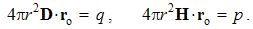 | (4.2) |
The full flux of each of the fields, evenly distributed in all directions, equals to respective charge – in the center. In a given solid central angle, the flux is independent of the radius of a concentric sphere, pierced by it. The division of the space into multiple such angles – with distinct radii, enables generalization of these two equalities to arbitrary surface embracing respective charges: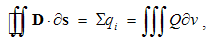 | (4.3a) |
 | (4.3b) |
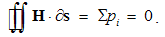
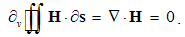
Here Q = ∂q/∂v is the charge volume density, and ∂s & ∂v – the small values of surface & volume. The scalar products take into account only the radial ∂s components.The surface integrals (at the left) are independent of the charge position, and the same procedure may be applied to each point inside the given volume. This possibility enables respective summations of the fields of arbitrary multiplicity of the contained charges. The set of these poles may be thus substituted by the sums or volume integrals of respective distributed charges, at the right sides of (3).The two equations may be commonly expressed: the field flux exiting a closed volume equals to respective charge contained in it. In the absence of free magnetic poles, the sum of their couples annuls, as well as respective flux of the magnetic field (3b). If the surface cuts a magnet ‘between’ its two transparent poles, the equal and opposite internal and external fluxes cancel each other.
4.3. Kinetic Laws
A moving charge forms the convection current, j = qv, equivalent to a short segment of the line current, j = Il, where I is this current, and l – the short conductor segment. With respect to the bound and transparent magnetic poles, respective current cannot be defined. Observing only its external field, a moving magnet may be approximated by two opposite magnetic currents. Each of the two currents is followed by the dissimilar EM field.Alike the static fields, strictly connected to their carriers – irrespective of their own motion, the kinetic fields also somehow follow respective convection currents, and so are determined in the same reference frames: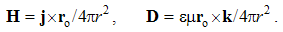 | (4.4) |
They are invariant only in these frames. Cross-product of a current and radius, as respective momentum, determines circular direction and sine distribution of the field along the polar angle between the current and radius.With respect to the circular magnetic field around a line current, (4a) is introduced. In the absence of such empirical basis, (4b) is the mere analogy. The former one is magnetic function of electric variable, and latter – all this opposite. The causal inversion is manifest by the product εμ and the opposite vector orders. The former distinction harmonizes the inverse relations of the electric and magnetic quantities, and latter – their vector relations.Their line currents, in the form of continual sequences of respective moving charges, will be obtained by integration. The axial integral may be substituted by equivalent one, in the polar angle θ – from zero up to π: | (4.5) |
Here I & K are the line currents (where j = Iδl & k = Kδl), and ρ = r sin θ – the cylindrical radius, as the transverse distance. A kinetic field circulated along concentric circle equals to the embraced dissimilar current. Alike fictional magnetic pole, respective line current is only the auxiliary concept, restricted to this consideration.The generalization of (5) into the integral laws is made in the cylindrical coordinates. The substitution of a circle by an arbitrary flat contour is similar to that at the static laws, but instead of solid, usual angles are here used. The field circulation along the arc of a central angle is independent of the radius, and the full angle may be divided into a number of angles with different radii. Their arcs together form the arbitrary flat contour, embracing the current.With respect to all the cross-sections mutually equivalent, the flat contour may be also deformed in the axial direction. Moreover, a line current may be substituted by respective current sum or the surface integral of its spatial distribution, as the field of electric current (J): | (4.6a) |
 | (4.6b) |
The displacement current (∂tD) – of bound electricity in dielectrics – is added to the current of free electricity (J), of the convection and conduction components. In the absence of free magnetic carriers, respective term in (6b) is reduced to the analogous displacement component.
4.4. Differential Equations
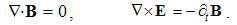
Integral laws express general field distributions around similar or dissimilar moving charges. They thus relate the spatial distributions of the charges and their currents with respective fields. Thus, the determination of the wanted quantities (on their left sides) demands the solution of the integral equations. Their application is thus restricted to the particular problems, one law – to respective problem. The clumsy graphical form of these laws hinders more complex formal procedures. For this reason, Maxwell turned them into – more operative – differential equations.There can be shown that volume derivatives of the field integrals (3) are equal to their divergences, thus giving the static pair of Maxwell’s equations: | (4.7a) |
 | (4.7b) |
The latter equation is confirmed by the vector-potential A, defined inversely – from the magnetic field: | (4.8) |
The mixed product, repeating a factor, annuls. This result of the differential calculus has already been interpreted at consideration of respective integral law.The similar derivatives of the kinetic laws (6) – per the transverse surfaces – represent their curls, thus giving the kinetic pair of Maxwell’s equations: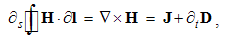 | (4.9a) |
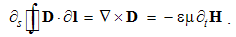 | (4.9b) |
The complete Maxwell’s set forms a table: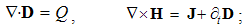 | (4.10) |
 | (4.11) |
The constitutive substitution in (7,9-b), of the rational – by respective force fields, the constants are eliminated from (11). By the similar – free and/or bound – EM charges, the static equations determine non-vortical, and – by respective currents of dissimilar charges, kinetic equations determine the vortical field components. The logic of the full set just points to its at least partial symmetries.Though mathematically equivalent with the integral laws, Maxwell’s equations are more operative. The clumsy are substituted by very concise expressions, applicable to the procedures as (8b) is. Instead of the full spatial domain observation, the carriers are located in the field derivatives, at each point separately. However, their final solutions are not localized at all. Though the two spatial derivatives are determined by given quantities at each point, they are not sufficient for the field determination. Apart from spatial derivatives in the whole domain, their own starting values on a boundary surface are demanded. A possible basic set, directly relating the given and wanted physical quantities at the same points of space, is wanted.
4.5. Summary
Apart from the rational fields, (10) contain the free terms, as the curriers. On the other hand, with the substitution of the rational – by force fields, the two EM constants are eliminated from (11). Obviously, the homogeneous form of this pair may be related with the absence of free magnetic carriers. Therefore, the rational fields are somehow related with the electric, and force fields – with magnetic carriers. Apart from the two distinct theoretical approaches, this conclusion points to mutually parallel electric and magnetic layers in the medium structure. The determination of a vector field demands its curl and divergence. Four Maxwell’s equations thus determine the two fields, i.e. the vortical and non-vortical components of each of them. However, the elimination of a symbol pair is not correct. Though the first and last equations concern the full electric field, the non-vortical component – from (10a) – cannot be directly related with the vortical field (11b). On the other hand, (10b) understands the variations of the full electric field. The trivial equation (11a) only speaks against possible existence of free magnetic poles.The wanted fields at left (10,11-b) depend on motion of dissimilar charges and on temporal variations of respective fields. In the same sense, temporal variations of the given fields are related with acceleration of the carriers dissimilar to them, but thus similar to the wanted fields. Therefore, the wanted fields are the indirect functions of some acceleration of the similar carriers. Apart from the kinetic, the dynamic senses of the two curl-equations are thus pointed at. In the absence of free magnetic charges, free electricity is moving in (10b) and accelerating in (11b). Therefore, the former of them is kinetic and latter dynamic equations.The relations of EM fields and carriers in Maxwell’s set may be interpreted in the two formally equivalent ways. In the standard opinion, EM fields (static & dynamic electric and kinetic magnetic) are determined and limited by the distribution and motion of the curriers. The material essence is thus ascribed to the particles, as the sources or carriers of their fields. On the other hand, the assumed particles may be understood as the formal features of the fields. Some separate material essences of the particles, distinct from their fields, are thus called in question.
5. Algebraic Equations
Algebraic equations relating the two EM fields express their interactions. The comparison of the static and kinetic fields gives convective actions, and substitution of kinetic, by dissimilar static fields – relative reactions. The roles of the carriers and their objects are symmetric. The addition of the fields nominally similar gives the mutual relations, and substitution of convective by local terms – hybrid equations. Some principal answers are still prolonged.
5.1. Introduction
Field carriers treated as the sources impose the question of the force transfer. The successive force transfer would understand the continual field expansion. A finite expansion speed would deform the emitted field around its moving source. However, nobody incorporated these deformations into Maxwell’s set. Instead of the transfer, the distance from the carrier is usually bridged up by its field, acting directly and continually in the whole domain, without any delays, irrespective of the object location. The transfer is thus not disturbed by the carrier motion.A theory tries to relate the finite speeds of a particle and expansion of its field. Instead of the clumsy mathematical expressions, this theory does not offer any palpable result, and has never been experimentally confirmed. In the final instance, longitudinal asymmetry of the expanding field, as the consequence, would call in question the uniform motion of free particles. Though disparate with his own equations, Maxwell’s principle was accepted in the package with them. The quantum theory thus explains the particle interaction by the exchange of some invisible photons.This disharmony of the principal views and equations of EM theory has not been clearly noticed, and as such is built into modern physics. Unlike quantum theory, assuming the photons, SRT is founded just on the quite opposite opinions. Negating the vacuum medium, it ignores any process of the propagation. In spite of this controversy, quantum electro- dynamics pretends to their unification. At least implicitly, Maxwell’s equations further understand the field action in the object location. The force delay is avoided by perpetual presence of the field in the whole domain.
5.2. Convective Equations
EM forces per unit objects are already expressed by the force fields (E & B), and so their consideration is reduced to determination of these fields. These two are proportional to the rational fields (D & H), obtained by the distributions of the similar static and/or dissimilar kinetic fields around the electric and/or magnetic carriers: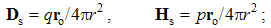 | (5.1) |
 | (5.2) |
Here j = qV is electric, and k = pU – magnetic current, with V & U as the charge speeds. The static fields are radial vectors, equal to the even distributions of similar charges around concentric spheres, and kinetic ones, proportional to the speeds of the dissimilar charges, are distributed by the sine of the polar angle. Irrespective of their own motion, the fields are determined in the carrier frames.With horizontal symmetry, vertical asymmetry of (1 & 2) enables the causal relations. The elimination of the charges, as the referent bodies, causally interrelate the two dissimilar surrounding fields, in the reciprocal ways:  | (5.3) |
These equations give the two kinetic, as the functions of the speeds of the dissimilar static fields. The former of them expresses magnetic action of moving electricity, and latter – electric action of moving magnets. The latter effect is well- known as EM induction. With respect the constitutive links, they are also expressed in the force fields: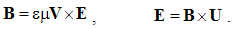 | (5.4) |
As at Maxwell’s differential equations, the use of (3a) & (4b) – with two field pairs, the two constants are avoided. The vacuum fields (H & E) depend on the motion of the total fields (D & B), respectively, speaking in favor of these forms. The total fields implicitly contain the influences of material media. The inverse dimensional relations in (3b) & (4a) are compensated by the constants.By superposition principle, the above pair, derived for the moving poles and their central fields, may be generalized to the arbitrary sets of the moving charges, as the convection currents. The generalization to the conduction currents, as mutual motion of the two opposite polarities, uses the same principle, but in the inverse direction. Although the moving electrons and their fields are statically compensated by the opposite resting quantities – of the lattice, their motion produces the dissimilar fields, independently of the resting polarity and its field. At ferromagnetic media, with some remnant magnetization, (4b) must be reduced to the moving components only of the magnetic field.
5.3. Relative Equations
The two fields given by their distributions and related by convective equations, act upon their objects by the forces determined by the laws of their actions. These laws are also needed for the final force determination: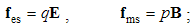 | (5.5) |
 | (5.6) |
Here j = qv is electric, k = pu – magnetic object current, and v & u – the speeds of the two moving objects. Unlike the similar charges, affected by the static forces – collinear with the fields, the dissimilar currents suffer kinetic forces, transverse to the currents and fields.This set represents a new basis for some causal relation of the two EM fields. With respect to the force equivalence, each of the kinetic forces may be substituted by equivalent dissimilar static forces. Vertical elimination of the forces and charges gives the relative equations: | (5.7) |
The moving carriers – from the convective equations – play the roles of respective objects. These equations thus express the reactions of the present fields on the motion of their dissimilar objects. By means of the constitutive links, they are also expressed in the rational fields: | (5.8) |
As formerly, the simpler pair (7a) & (8b) is usually used. It expresses relative reactions of dissimilar EM fields, equal and opposite to the convective actions.The sums of the nominally similar fields, convective and relative ones, superimpose the kinetic actions and reactions between dissimilar moving charges: | (5.9a) |
 | (5.9b) |
These equations express the same force sums of kinetic interactions of two dissimilar moving poles. In the terms of electric field, the former is the difference of the magnetic action and electric reaction, and latter one – all this opposite. With respect to the lack of movable magnetic objects, the former equation only is usually used.The active fields of the two dissimilar moving charges are directed along their distance, with the zero products and respective forces in their longitudinal motion. The Fig. 1 thus presents their transverse motions. The opposite forces, dependent on the same speeds, confirm the action-reaction symmetries. In the case of the equal speeds, the dissimilar forces affecting the same poles annul. 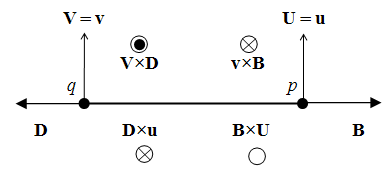 | Figure 1. Convective and relative inductions |
In the more real physical interaction, of an electric pole and magnetic dipole – perpendicular to their distance, the longitudinal motion is also relevant. The symmetric mutual motion causes the same forces on each of the two charges, irrespective of its own motion. This geometric symmetry explains the algebraic force anti-symmetry (9). This is also the case in Maxwell’s curl-equations.
5.4. Hybrid Equations
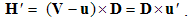
At the mutual interactions (9), the moving static fields act directly, as the convective actions. Their products with the object speeds, as the reactions, are added. The equations (9) are thus expressed in the following form: 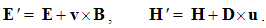 | (5.10) |
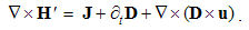
The algebraic and differential equations are derived from the same central laws, and so, their direct relation may be expected. Via convective derivatives of EM fields – in the lesson 11, these relations will be confirmed. Therefore, the convective field actions (E & H) may be also expressed by the two Maxwell’s curl-equations: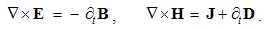 | (5.11) |
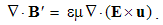
The inductions arise at resting points, caused by variation of the moving fields. Curls applied to (10), with the former terms substituted by (11), finally give: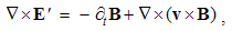 | (5.12a) |
 | (5.12b) |
Respective div-pair can be added to them. Div applied to (10), with substitution of the div-equations, gives: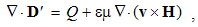 | (5.13a) |
 | (5.13b) |
Magnetic divergence (13b), as inverse relative induction, is the reaction of the present electric field to the motion of magnetic poles or dipoles, as the objects.If, instead of the two dissimilar poles, a common detector were moving through their resting fields, the results would be also described by (10), with a new interpretation. Apart from the common speed (u = v) – in the relative terms, the convective would be substituted by the primary fields. Thus obtained field transformations express the forces affecting the objects in the moving frame, connected to the common detector. These transformations will be further considered in the two future lessons, i.e. 11. & 16.
5.5. Summary
The convective algebraic equations express the effects of rectilinear motion of the given, implicitly rigid, EM fields. Not only that they have not been so far generalized to the rotated and deformable moving fields, but the cases of such applications fall into some difficulties. These facts impose the restriction of their validity to the translation of the rigid fields, stably oriented in the space. Some of their specific applications – in lesson 10, as well as their direct relation with Maxwell’s equations – in lesson 11, will explain these restrictions. With these formal limitations, the empirical verification of the algebraic equations is hindered. This was the main reason of their less affirmation.Despite, almost all here presented algebraic equations can be found in various text-books, separate or included into the complex equations. Not only that they are nowhere thus systematically derived, arranged and mutually compared, but they were in the start subdued to one of the two doubtful complication: the field delay behind its carrier or relativistic correction of the transverse components. These two formal complications can be temporarily bypassed, and respective theoretical dilemmas avoided. Moreover, they both will be finally disproved in the future lessons.The assumed delay of the expanding field of a moving charge relies on a Maxwell’s thesis, disparate with his own equations. Not only that the modern concept of the photon barter is not convincing, but it cannot anyhow explain EM forces. With respect to the experience, the particles manifest by their fields, and interact by these fields. There is no any proof of existence of a solid particle body, distinct from the field. In the final instance, the field is the part of its particle, or the particle is only the center, something as a knot of its field. The convective equations thus describe the direct field actions, in each point of space separately, irrespective of the assumed material sources or carriers.With respect to their derivation hare already presented, Maxwell’s equations do not at all include the relativistic field correction, otherwise directly imposed to incomplete field transformations, for the sake of their own ideal form, without any empirical basis. Its roots will be presented later. There is sufficient to say that some field corrections are not any effects given in advance, but express the proper kinetic interactions, founded on application of the mutual kinetic interactions here presented. Though statically superimpose to the primary fields, they do not move with these fields and do not disturb the basic equations. Otherwise, their motion would cause a sequence of the kinetic effects. Not only that these effects are logically unacceptable, but they have been never empirically noticed, and cannot be.
6. Constitutive Relations
General theory of physical quantities is here applied to electrodynamics. Gradual elimination of temporary physical constants and reduction of the basic set are presented. The optimal system of physical quantities and measuring units is thus looking for. The known such systems of the physical quantities are presented and classified with respect to their formal symmetries or rationalities. The two fully exhausted dimensional reductions are finally compared.
6.1. Introduction
Various quantities, as the basic notions of physics, are mutually related by respective laws. In the final instance, the complete development of physics may be reduced to the gradual introduction and mutual relation of such quantities. Each law relates at least two, and each new introduces at least one quantity. The number of quantities thus exceeds at least for one the number of the laws. In the general case of a scientific system, for mutual relation of its n notions, n – 1 relation is necessary and sufficient. With the less number of relations the system is not determined, and with greater – it is pre-determined. In these cases, the laws still unknown are looking for, or a mutual collision or equivalence of already known laws is re-examined, respectively. Possible introduction of a new physical law is usually performed in the two ways: as the definition of a new, or empirical relations of the known physical quantities. The definition of each new quantity, in the form of an algebraic relation, directly relates the new with old quantities. On the other hand, empirical correlation of already independently introduced quantities cannot establish the equality, but only the proportionality of the expressions on two sides of the equations. Therefore, the empirical laws are harmonized dimensionally and numerically by the temporary constants. Unlike the mere definitions, as the rational relations, the empirical laws contain physical constants.The quantities still not related directly constitute the basic set of the quantities or physical dimensions. Their algebraic combination gives all the remaining, derived quantities. By direct relation of two basic quantities, one of them would be transferred into the derived set. Thus excluding all derived set and respective definitions, the basic set exceeds by one the number of the basic laws. A greater difference demands further elaboration of the theory or its interrelation with other physical theories. At the zero or negative difference, the reexamination and comparison of the basic laws enable the elimination of their excessive number.
6.2. Quantities & Constants
By elimination of their physical constants, empirical laws are turned into rational relations. With respect to scientific experience, final rational essence of all the physical laws is expected. On this basis, the majority of physical constants may be neglected in advance, reducing them to the units or other convenient numerical values. A consistent physical theory, with the unit difference of the numbers of the basic quantities and empirical laws, would be thus reduced to only one basic quantity, as the final unique notion of the theory. However, such the formal reductions are usually in conflict with the phenomenal distinctions, or with – by the time established – scientific prejudices.As the typical example, classical mechanics was initially founded without gravitation. Though introduced empirically, force action law is formulated in its rational form, without any constant. This law directly defines and harmonizes the force by the three basic quantities: mass, length and time. However, in the law of gravitation force is not in harmony with mass and length, without time. The consistent harmony, by elimination of gravitational constant, would reduce the basic set to the two quantities. Therefore, even extended by gravitation, mechanics is not a complete scientific system. There follows its interrelation with electrodynamics, in this aim conveniently founded on respective central laws, easily comparable with the laws of mechanics. Initial introduction and mutual relation of EM quantities, irrespective of the mechanics, started by the two static laws. In their empirical forms, these laws contain the constants (a & b). Apart from the needed numerical and dimensional harmonization, the two constants determine the influence of material media on EM forces. The two roles are separated by the factorization: a = arao & b = brbo. Here the relative factors express medium influences, the dimensions of the vacuum factors define two EM charges, but their numerical values harmonize the measuring units.Before kinetic relation of EM phenomena, Gauss adopted the unit values for the both vacuum factors, ao = 1 = bo, with dimensional equality of the two charges: p (=) q. Derived from force and length, the charges were expressed by the basic mechanical quantities. By later kinetic relation of EM phenomena, the ratio of the two constants or their vacuum factors is consistently established: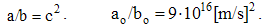 | (6.1) |
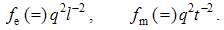
Here c is the speed of light propagation. Alike the two EM constants, it is also factorized (c = crco), with respective mutual relation of the three vacuum factors (1b). With respect to the known equality, aq2 (=) bp2, (1b) also relates dimensionally the two charges: p/q (=) co.Via the action of a charge, as the carrier, onto another – as the object, the two force fields (E & B) are introduced. On the other hand, starting from EM charges, as the field carriers, rational fields (D & H) are defined. The similar fields are related empirically: D = εE and B = μH. The former definitions, substituted into these relations, relate the old and new constants in the inverse sense: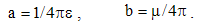 | (6.2) |
The new constants are symmetrically related with speed of light: εμc2 = 1. They are also resolved into the relative and vacuum factors: = εrεo = μrμo. The former pair expresses the medium features, and latter determines the physical dimensions and units. At vacuum, as the etalon medium, with the adopted unit relative factors, the two EM constants reduce into their vacuum factors.Unlike the set of central laws, the algebraic and analytical equations represent the basic laws of EM field theory. Expressed by the two field pairs, they are free from the two constants. In the consistent dimensional systems at least, their forms are invariant. If the two field symbols were eliminated, the constants would appear in the basic set, thus slightly disturbing its formal invariance.
6.3. Asymmetric Systems
With respect to the relation (1b) of the vacuum factors, with formerly introduced and habituated basic units, only one consistent value of each Gaussian convention is correct: ao = 1 or bo = 1. The two systems are thus introduced: static and absolute. The force is thus defined twofold, by electric,  , or by magnetic factors,
  :
: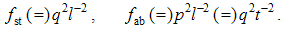 | (6.3) |
With the equivalence understood, EM and mechanical forces are equaled. Electric charges are expressed by the fractional exponents of mechanical quantities: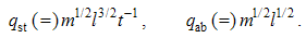 | (6.4) |
The same quantities in the two systems stay in the ratio co, but symmetric ones are of the same dimensions. The static capacity and absolute inductivity are thus expressed by the length. The above fractions can be avoided by electricity – instead of mass – as the basic quantity.Apart from fractional exponents, these systems disturb the vacuum factors by the constant 4π: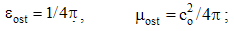 | (6.5) |
 | (6.6) |
Entering the basic laws, they disturb the equations. With respect to the obvious cancelation of 4π- in the relation  = 1, this constant may be missed in advance from (5&6). Measuring units of thus obtained system would be scaled by
  . However, the further development took the two other ways – in the two directions.For the needs of technical practice, the absolute system is a little modified. With the inherited mechanical quantities, electric charge (or line current) plays the role of the fourth basic quantity, with the unit ten times smaller than absolute one. The two factors (6) assume their own artificial physical dimensions. The translation from the CGS into MKSC units also changes their numerical values:
 | (6.7) |
The symbols of the two factors – in the basic equations, instead of their numerical values, give the impression of their rationalities. Even by the force, instead of mass, as the basic quantity, the fractional exponents are not eliminated. Thus ignoring the dimensional relations with mechanics, in relatively independent technical practice of the two physical disciplines, the number of the basic quantities is increased. Habituated in the practice, this system is established as the international technical standard (SI).
6.4. Symmetric Systems
Looking for more consistent dimensional solutions, with keeping the inherited mechanical units, Heaviside proposed the same value of the two vacuum factors: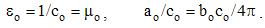 | (6.8) |
With respect to the equality,  , Maxwell’s curl equations at vacuum take the anti-symmetric forms:
 | (6.9) |
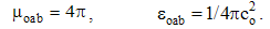
As such, they were used in SRT, known by the similar artificial symmetries. As if, these equations point to the forth metrical axis: x4 = cot. Apart from material media, this system is not convenient at central laws (8b).Mentioned Gaussian system, with the unit old factors, is not symmetric with respect to the new factors: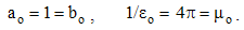 | (6.10) |
In a quandary about the vacuum fields (E & H), 4π was applied to the material components (P & M) only. The mix of the static and absolute units was used.The fully consistent natural system (NS), with symmetric elimination of the new factors, obtains also the symmetry of the old vacuum factors – in central laws: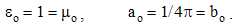 | (6.11) |
With the same physical dimensions as in GS, NS scales the units by the constant  . For this reason, it is neither widely applied nor habituated in practice.NS demands radical revision of the dimensional relations. With respect to the equality
  , without dimensions of the two factors, time is directly reduced to length: t (=) l. On the other hand, the comparison of mechanical and EM forces, as the actions and reactions, their direct relation is established: m (=) q2l–1. The basic set is thus diminished from four to two remaining physical quantities.
6.5. Summary
The metrical time also reduces some derived quantities. The energy and momentum are reduced to mass, and power – to force. The two EM fields obtain the same dimensions, enabling their quantitative comparison. The two vacuum fields at EM wave are thus equaled. Their static exclusivity and phenomenal distinctions are explained by their distinct positions in 4D space. NS is convenient in the field theory, especially – in the 4D space. In electric circuits, however, it equals dimensionally the voltage and line current. Though thus unified, these quantities can keep the distinct names of respective measuring units. This may be also the case with the mechanical quantities already equaled.There remains the final reduction to a unique quantity. Missing the law of gravitation, modern physics eliminates the Planck constant, from the expression of a photon energy: w = hν = ħω. With the metrical time – from EM reduction, mass turns into inverse length, but electricity losses its own dimensions. Apart from the irrational law of gravitation, this reduction exceeds the frames of classical physics. Let us so consider the final classical reduction.Mechanical & EM theories are founded on the four basic laws, by two each of them. After the initial reductions, they relate the fifth quantities: the two kinematical and common force, with mass and electricity, as the two basic substances. Really, 5 − 1 = 4 accords to the number of the basic laws, thus enabling the final reduction. The elimination of all the constants gives the following equalities: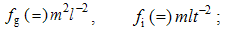 | (6.12) |
 | (6.13) |
EM static laws are added to the laws of gravitation and force action. With the zero sum of the exponents in each force, there is the obvious final solution: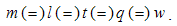 | (6.14) |
With dimensionless force, all basic quantities are unified. The same dimension also belongs to energy.Elementary charge or Planck constant may be accepted for the universal unit: e = 1 or h = 1. With respect to the probable implicit relation of these two constants, the two distinct dimensional solutions would be thus finally unified. Some interpretative consistence would demand the constant 1/4π in the law of gravitation, with the new constant: g = 4πγ = 1. And finally, the elimination of Boltzmann constant is also understood: w = (k)T. In fact, temperature is noting else but the average molecular energy.
7. Absolute Laws
Two approaches to the field theory are here presented and compared, starting from the continual quantities or the discrete structures. By volume derivatives or zooming of a structure, it is stratified into a sequence of structural layers, along structural dimension. EM processes are thus observed in the four such layers. Two absolute laws are formulated and explained on this basis: of electrical neutrality – in 3D, and of energetic homogeneity in 4D spaces.
7.1. Introduction
The classical field theory initially started by two opposite, mutually equivalent approaches. The initial idea of the force fields was demonstrated by the chains of material scrapings surrounding EM charges. General notion of physical fields, as the quantities distributed in space, has been consistently carried out in the mechanics of fluids and deformable solid bodies. Unlike the fields distributed in space, their integral sums reduced to a point we call discrete quantities. On the other hand, starting from the known or assumed structure, the fields may be introduced statistically, as the scalar or vector densities of the discrete quantities.One of these two approaches is used, at least formally distinguished by the field symbol conventions: lower cases – in the continual, and capitals – in statistical treatments. They represent the two approaches: from a body – towards its continual density at a point, or from elementary particles – towards their statistical concentration. At least implicitly, the kinematical fields of displacement and speed are used in EM theory. By the distributed speeds, algebraic equations are formulated. The kinematical quantities turn directly into respective fields, of the same dimensions.Substantial fields – in the both approaches – are obtained by volume derivatives, with the dimensional division by l3. Algebraic combinations of these few types give the rational fields, as if contra-variant with respect to the radius vector. They are confronted by the force fields, as the gradients of respective potentials, as if covariant – in the same sense. Without any physical distinction, this classification in fact appears as artificial. And finally, the volume derivative of a field equals to zero. This is especially so in the case of the kinematical fields or respective quantities.
7.2. Structural Dimension
The forms of physical laws announce a fifth dimension, independent of the kinematical four. Similarly to the fourth – temporal axis, an uncertain fifth dimension was suggested a century ago. However, without any convincing physical interpretation, this proposition could not be widely accepted. The same idea is renewed later, assuming the circular fifth axis, closed into itself on the level of elementary particles. The absence of its visible manifestation is thus justified. This idea is followed by formal introduction of a sequence of new axes, without any scientific criteria. This is finally crowned by the string theory, founded fully speculatively, without any empirical or theoretical bases.The fifth axis we here introduce by volume derivative or the structural zooming. The extension of attention – from the structural depths towards cosmic widths, independent of space and time, may be understood as made along the two fifth axis legs. A physical point ∂v, as the minimal relevant volume in observed domain, determines the position on the fifth axis. A structure transformation, as its resolution into finer, or collection into cruder structural parts, displaces the attention along the structural axis. This is presented by 5D continuity equation: apart from the spatial sources of a substance and temporal variations of its density in 3D, the substantial term expresses its transformation.Some manifestations of the fifth axis are already known. 1.) The chemical and nuclear processes develop in parallel, inside the same material. 2.) At ionized gases, as the mixes of various particles, the particular components are observed separately, as respective independent gases. Apart from their various charge and mass densities, the pressure and temperature of each of the components is treated nearly separately. 3.) The particles of material structures occupy their – strictly exclusive – quantum levels. Tunnel effect, as unobstructed passage of some particles through the material, is thus realized on the free quantum levels. 4.) In the final instance, these examples remind the parallel worlds from the mystical stories or science fiction.In the case of EM phenomena, material structures may be divided into the four operative layers: apart from a vacuum, that of the polarization, magnetization and conduction. The finest layer is manifest by the two vacuum fields: E & H. The next two represent the substrates of the material fields: P & M. The last layer concerns conductors and free space, with free electricity (Q) enabling conduction or convection currents (J). Only the first medium layer is omnipresent, but remaining ones represent the local material situation. EM processes may be restricted to one or more layers. Their diffusion into other layers, as the motion along the fifth axis, enables the ‘vertical’ communication.The systematic reduction of physical quantities may be also related with 5D space. After elimination of the two EM vacuum factors, the speed losses its physical dimensions, thus dimensionally equaling length and time. With direct relation of the mass end energy, the two EM fields are also mutually equated. The final elimination of the gravitational constant equals all the basic quantities, thus terminating the process of their gradual reduction. Formal equivalence of substantial and kinematical quantities demands a fifth axis, just representing the structural dimension.The position on the structural axis is limited by the size of the elementary particles in the observed structure. In the mathematical sense, these particles just accord to a physical point ∂v, as the minimal relevant volume. This volume is determined by its radius, and its own logarithm gives the two axis legs, each defined from the zero up to infinity. One of them just strives into structural depths, and the other – into cosmic widths. The zero of the fifth axis itself is strictly determined by the adopted common unit.
7.3. Electrical Neutrality
Scalar physical quantities, stable under some conditions, we call physical substances. Their particles are the objects of the physical forces, dependent on kinematical quantities. Unlike the non-polar substances, as mass is, electricity is a bipolar quantity, consisting of the two opposite polarities. Unlike the mass, at least conditionally conserved – in the absolute sense, electricity also saves the algebraic sum of its two polarities. By mutual attraction, the opposite polarities mix with each other, thus forming the neutral structures. This tendency in each particular and more structural layers is expressed by the static laws of EM theory.The free electricity Q2 – located in the conducting layer, repels the equipolar and attracts opposite polarities from the dielectric Q1 and vacuum Q0 layers. The repelled polarity forms the flux of electric displacement through each closed surface, but the attracted one compensates the initial charge. These two processes taken together point to the perpetual maintenance of neutrality at each 3D point: | (7.1) |
Here Qi = ∂vqi is charge density, as a polarity in the layer. The index (i) concerns the observed structural layer and respective volume derivative. The pure vacuum is ever neutral, but – at the disturbed material media, its electricity compensates the algebraic sum of the disturbances in the two material layers. The disturbance of the conducting layer is proportionally compensated from the two dielectric layers. The opposite strains in the structural layers point to the force balance at each point of 3D space.In the classical laws, restricted to one or more layers, the electric charge statically manifest is observed, distinct from free or bound, mutually opposite polarities. This distinction of the two quantities demands a separate symbol for electric charge. However, with respect to the total neutrality, each such charge is also compensated by the opposite polarity from the same or the other layers. The need for the separate charge symbol is thus overcome. As the electric current in Maxwell’s kinetic equation understands the motion of a polarity, irrespective of its manifestation, this is the same case in the static equation. Though statically compensated, the moving free electricity carries by itself its electric field, statically un-manifest in the experience.Presented introduction of the law of neutrality relies on the classical electrostatic laws, confirming its equivalence with these laws. On the other hand, the new law is the direct result of the known Faraday’s experiment. Some charge entered into a closed metallic sphere causes the polarization of the surrounding medium, including the vacuum medium and the walls of the metallic sphere. The external surface thus obtains the charge of the entered polarity. Faraday also established their quantitative equality.
7.4. Energetic Homogeneity
Force action law will be derived from EM interactions, with the law of inertia, as the special case. Apart from the law of gravitation, introduced separately, there remain the laws of the force balance and work performance: | (7.2) |
The former law relates and dimensionally equals various confronted forces, and latter defines the energy accepted by the reactive force. The energy transfer also describes the same interaction, alternatively to the force used at the initial foundation. Though needed for the energy introduction, (2b) is not treated as the basic law. Its inversion will exchange the two roles of these two interactive quantities.The law (2a) usually expresses the static balance of two forces: action and reaction. By superposition, this relation is generalized to multiple such forces or their components. Static balance of a resting point is expressed by zero sum of all engaged forces. After introduction of the frictional and inertial forces, the balance is generalized to the kinetic and dynamic processes. Via the object moved by an action, the performed work equals to the energy accepted by reaction (2b). The positive sign with the active force – in the same law, represents the energy investigation.Volume derivatives of the discrete quantities in (2), in the same manner relate respective physical fields: | (7.3) |
Instead of the discrete quantities, there are their volume densities, as the fields. These force fields act in respective structural layers, with the vertical transfer of energy. The displacement ∂R = ∂r, as the kinematical quantity – equal to the field, is not subdued to volume derivative.The direct comparison of (3b) with the total differential of energy (4a) gives the inverse relation (4b): | (7.4) |
According to it, the energy density is the potential of the force field. On the other hand, the zero sum (3a) points to the homogeneous density of the total energy: | (7.5) |
The sum of gradients equals to the full gradient. Though homogeneous in some structural layers, various components supplement each other up to the full sum.The division of (3b) by ∂t gives the derivative of energy density, as the power field of its vertical transfer: | (7.6) |
Temporal derivative of the stationary force field annuls. The power field represents the density of the energy transfer between two layers. The equality of invested and accepted energies, or zero power of the closed compositions, may be treated as the energy conservation in 5D space.As the typical example, Bernoulli’s equation expresses the energy density maintenance, consisting of gravitational, kinetic and thermal components:  | (7.7) |
The last component is manifest by the pressure: P = Nw, where N is the particle concentration, and w = kT – the average thermal energy of a particle, and T – the absolute temperature. The macro-speed of the fluid flow (V) can be increased by the loss of height (H) or by the rearrangement of the chaotic particle motion. The last transfer is manifest by the reduced transverse pressure (P).
7.5. Summary
The principle of impenetrability excludes the coexistence of two solid bodies in the same 3D location. This principle at fluids is displaced along structural axis, from the bodies – to their molecules. The coexistence of electric and magnetic fields is explained by their distinct subspaces in 4D. The principle of superposition also understands the undisturbed coexistence of many similar fields, with effective addition of their effects. Faraday considered that the field of each particle occupies the full cosmos, in parallel with other such fields. This view precedes Pauli’s principle of an exclusive quantum level assigned to each particle.With respect to the above views, structural dimension is already implicitly used in physics. Explicitly thus named, it is now widely and systematically elaborated and formalized by the volume derivative. Its consistent application enabled us the formulation of the two absolute physical laws: of electrical neutrality and energetic homogeneity. Respective classical laws, as their particular versions, express the same tendencies in one or more structural layers. The particular medium disturbances just express the material structures. Their annulment would mean the factual eradication of the phenomenal world. Let us now consider in principle the body motion in the frames of this world.At motion of a body or particle, with its field and energy, the gradients of these quantities in the body front and back are also thus moving. With respect to energy homogeneity, the moving energetic image in a layer is followed by its negative complement, in the other structural layers. As if, energy circulates between the two layers. A moving entity accepts the energy in the front, and releases behind itself. This process will be described in detail around a moving charge. It just resembles the water waves, where the vertical oscillations give the impression of the horizontal motion. In the final instance, some philosophers negate any material motion, reducing it to the sensory illusion.
8. Material Media
By volume derivatives of the sets of structural elements, three rational fields – displacement, current and magnetic – are introduced, as respective three functions of the position, motion and circulation of electricity. With some reliance on fifth axis, principle of neutrality and EM inertia, Maxwell’s equations are also confirmed and constitutive relations – extended. The closed forms of all EM fields, in space, time and medium structure, are established.
8.1. Introduction
Standard presentations of EM theory treat vacuum before material media. Such approach does not give sufficiently transparent exposition, thus annulling its methodological advantages. The mutual relations of partial descriptions are not sufficiently clear. Some authors introduce the particular Maxwell’s equations, for the bound electricity at dielectric media. The universal sense of the standard equations is here shown, but these additional appear as excessive at least, or importing some confusion in the theory.Apart from the mutual relation of various quantities, the connection between temporal variation and motion of the same substances is of interest. In this sense, let us consider a scalar field N, as the particle concentration. In the interval between their formation and dissolution, their concentration is correlated with motion through 3D space. In principle, this is described by 4D continuity equation: | (8.1) |
The observed substance running into or out of a given location is described by divergence of its current, consisting of three components. This process is followed by respective variation of its local density (N), expressed by the temporal derivative. In the aim of taking into account its formation and dissolution, a substantial term must be added.
8.2. Displacement Field
We observe three electrical structural layers: conduction, polarization and vacuum. Irrespective of its initial cause, each primary disturbance further causes some displacement of electricity in the medium, Di = QiLi, where L is vector field of the spatial displacement. This is valid for each layer (i) – separately, or for more of such layers in common. The introduction of electric displacement starts from the dipole, p = ql, as respective structural element. Vector density of a set of such dipoles gives respective field: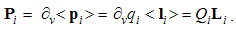 | (8.2) |
There is understood that each physical point (∂v) contains a great number of the elementary dipoles. The kinematical displacement field L = <l> behaves as the constant along the fifth axis, with the zero volume derivative. At external field E, the displacement is divided between the vacuum and material structural layers: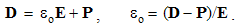 | (8.3) |
The constitutive relation (3a) directly gives the vacuum factor (3b), as the ratio of the collinear field components. On the other hand, the relative factor is the ratio of the full and vacuum displacement field components: | (8.4) |
From the adopted unit – at vacuum, the relative factor is usually greater – at dielectrics, and may be considered as infinite – at relatively good conductors. The product of the two factors gives the full electric constant, as the ratio of the displacement and electric force field.The electric displacement of one medium polarity is also manifest by the remaining opposite charge. In the final result, the lines of displacement field start from a negative, and terminate on positive polarities. This is expressed by the static continuity equation: 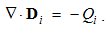 | (8.5) |
Here Qi is the charge density in a layer. Due to the total neutrality (Qtot = 0) the displacement is closed: 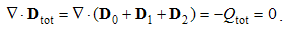 | (8.6) |
The opposite non-vortical fields in various layers close into each other, giving the unique field closed into itself in the frames of 5D space. The displacement of free electricity is usually closed by bound electricity of the two dielectric layers. In this sense, the three displacements give the two forms of Maxwell’s static equation: | (8.7) |
 | (8.8) |
These results are convincingly explained: free charge Q2 is the source of the full field, D = D0 + D1, but the source of the vacuum field, D0 = εoE, is diminished by the opposite bound electricity Q1 – in dielectric structure.
8.3. Current Field
A moving electric pole forms respective current: j = qv. In the statistical sense, volume derivative of multiple such currents gives the current field: | (8.9) |
Here v = V is mutual speed, as the relative motion of the two polarities. At least formally, discrete current accords to the temporal derivative of a dipole: j = ∂tp. If the density of the movable polarity were considered invariant, respective two fields are in the same ratio. The field V expresses the arranged motion or the vector sum of the statistical speeds in the full set of such elementary charges.The conduction current in conductors is determined by Ohm’s law, J = σE, as the kinetic relation. With respect to the known static relation, D = εE, the displacement is substituted by the current, and the static (ε) – by kinetic (σ) constants. The displacement currents are restricted to the transitional processes, compensating the static equilibrium disturbances, caused by external influences. Temporal derivative of (5) gives the kinetic continuity of current, as the non-vortical field in a layer: | (8.10) |
The current of free electricity, in conductors or free space – irrespective of static compensation of the two polarities, cause the variation of the local charge density.Unlike the non-polar substances, with the same scalar fields in both terms of (1), the continuity of electricity, as the bipolar substance – in (5) & (10), relates the left moving electricity – with right electric charge. With respect to the movable electricity hidden in respective symbols, in fact only one symbol (Q) is sufficient. Moreover, with respect to total neutrality, each charge is compensated. In accord with the relation of the polarization and current, the temporal derivative of (6) just gives: | (8.11) |
Apart from space and time, the fifth axis concerns the three layers. Though being non-vortical in particular layers, the current is closed into itself in 5D space.Unlike convection and conduction, displacement current appears in non-conducting structural layers: | (8.12) |
As the capacitive continuation of conduction, this current concerns the bound electricity. The motion is expressed by the two terms concerning the scalar field Q:  | (8.13) |
The former term means convective variation, and latter – dilatation (extension or compression) of Q. Its phenomenal variations result from its linear motion and/or deformation. In a stationary current, these two terms are opposite, and so cancel each other: ∇J = 0. At the two homogeneous fields Q & V, they both annul separately.
8.4. Magnetic Field
Magnetic dipole is the basic element of respective field. Its phenomenal definition, m = pl, analogous to the electric dipole, satisfactorily treats only its behavior in the external fields. The absence of free magnetic poles and the vortical field form, obstruct the wider application of this concept. The analogy with electric dipole does not speak in favor of their unification or reasonable mutual relation.Algebraic relations of EM fields point to possible similar relations of the two dipoles. In the absence of free magnetic poles, only one relation is possible. The rotation of electric dipole around one of its poles, as the current momentum, can be described by a chain of few equations: | (8.14) |
As the current momentum, this is magnetic dipole. At electric circuits it is defined as the product of the contour current and the surface embraced by it. At circular motion of electricity, without the central pole and its field, this gives a half of the value obtained by (14).Volume derivative of (14) turns the discrete quantities into respective fields, in the similar chain: | (8.15) |
Though mutually equivalent, these expressions point to three technical sources of magnetic field, with respective – practically distinct – physical interpretations.First definition describes magnetic medium, equal to the volume derivative of respective dipoles. The magnetization consists of the product of density of rotating electricity with the set of kinematical momentums (t = l v): | (8.16) |
After cancelation of the opposite adjacent micro-contours, there remains the current wail on the cylindrical magnet cover. This is equivalent with the current in a technical coil. The second field definition (15) thus expresses the circular currents and their magnetic fields.The third definition observes a moving polarized body, as the field source, e.g. a rotating cylindrical capacitor. The polarization of its electrodes, P = D2, is opposed by medium displacement: D0 + D1 = D. The final result accords with the equation: H = V × D. The rotation of the radial polarization gives the axial magnetic field, or vice versa.Continuing the magnetization, the external field springs from one, and dip into opposite bases. Taken together, these two in common form a unique magnetic field: | (8.17) |
The former equation expresses the field continuity on the two bases, and latter – the current veil on the cylinder cover. The present magnetization is also added: | (8.18) |
The ratio of the full and vacuum disturbances, as the two collinear magnetic fields (b), defines the relative magnetic factor. At vacuum adopted as unit, this factor is smaller in diamagnetic and greater in paramagnetic media. In non- linear media it is determined as respective function of the initial vacuum field (H). Mutually inverse definitions (4a) & (18b) secure that – in the predominant technical practice – both these factors are greater from unit.Various components add in same domains, and so (17a) is valid for their sum and the total field: | (8.19) |
The constitutive relation gives the vacuum factor, as the ratio of the force field and full disturbance: | (8.20) |
The product of the two factors gives full constant, as the ratio of the two collinear magnetic fields.The resolution of total electric current, according to (11), turns (17b) into Maxwell’s kinetic equation: | (8.21) |
The two former terms form the displacement current (12), and latter – the convection and conduction ones.Magnetic field arises at circulation of electricity, and its variations – at accelerated circulation, opposed by inertia of electricity, as the dynamic electric field: | (8.22) |
This is Maxwell’s dynamic equation, otherwise obtained from Faraday’s law (10.1b), as the empirical fact. The EM inertia will be elaborated in the lesson 13.
8.5. Summary
Though the magnetization need not be closed into itself, the complete magnetic field is opposite inside and outside a magnet. As the disturbance of one structural layer, magnetic field is closed in 3D, without non-vortical components. On the other hand, though the current components, irrespective of their layers – may be non-vortical, respective total field is closed into itself along the fifth axis. Therefore, all EM fields are somehow closed into themselves.EM processes start in a layer, by disturbance of structural electricity. However, the answers of other layers distinguish in the electric and magnetic fields. NS constitutive relations point to the former aspects of this asymmetry: | (8.23) |
As if the two forces are defined in the distinct layers: the electrical is formed in vacuum only, but magnetic concerns the material layer too. This is in accordance with respective elementary interactions: equipolar charges mutually repel, but parallel currents attract each other. The inverse vacuum factors further import the additional asymmetry: Unlike the electric medium disturbances, as the causal consequence of respective force field, magnetic disturbance is just the cause of respective force field. All Maxwell’s equations are here derived once again. Unlike their former derivation, by gradual generalization of central field distributions, this one clearly emphasizes their physical essences. The procedures are mainly based on the structural dimension and electrical neutrality, thus affirming these two fundamental physical concepts.
9. Moving Media
There are elaborated the convective inductions around moving bodies polarized by external fields. Their associated fields are scaled by the fractional factors, and their motion produces the convective effects. The same factors determine the wave drag by the moving media, manifest as the vector corrections of the energetic currents. The stratification of vacuum medium between massive celestial bodies and their gravitational potentials is finally explained.
9.1. Introduction
A material or vacuum between the active bodies – as the field carriers or their objects, represents the medium of EM processes. All material structures, in the solid or fluidic states, are plunged into the omnipresent vacuum medium and respective EM fields. By the static induction, the additional layers are thus polarized and/or magnetized. At continual, homogeneous and isotropic media, the induced fields are collinear with primary components, thus forming the final fields, in the same geometric forms. The irregular media deform all the components and final fields. All these effects impose some formal complications.At such media, the primary and final fields are related by tensors. The media in the form of solid bodies, limited by boundary surfaces, are the special cases of the irregularities. Unlike fluids, filling the full space and running in between, the boundary surfaces of solid bodies divide the medium into the internal and external domains, with the distinct features (εμ). The induced and associated fields depend on these features, as well as – on the surface shape. The most general considerations are thus developed into the complex theories of the technical boundary effects.The algebraic equations treat the convective and relative processes, caused by motion of EM fields or their objects. Their speeds are related to the assumed medium, or – to the nearer visible and palpable material surroundings. In such locally predominant medium, its own motion has not been here treated. In the meantime developed theory enables the treatment of the simpler cases of moving media and their effects. This is directly related with orientation of physical processes in space, in the sense of the determined reference frame concerning the observed motion. This is a first step in the approach to this complex problem.
9.2. Fractional Factors
In the observed domain of EM fields and their objects, let us consider a third body, as the medium limited by its own surface and moving in relation to some, locally preferred, as if hypothetical frame. In the first approach to this matter, we will restrict to the motion of material layers, forming the medium structure. The consideration is thus resolved into two successive phases, of the static and kinetic inductions. Each of these phases observes in parallel the independent electric and magnetic processes, by means of respective, mutually independent, algebraic equations.A present body is polarized by primary, forming material fields. They are determined by the given primary fields and respective medium features, expressed by the two fractional factors – dependent on relative ones: | (9.1a) |
 | (9.1b) |
The confusing asymmetry of these SI relations, imported by vacuum factors, disabled their notice. The symmetry is more convincing in the natural form (NS): | (9.2a) |
 | (9.2b) |
In the case of the medium boundary surface transverse to the primary fields, respective material fields, of the same forms and directions, are statically induced in the medium. These internal fields are continued in the surrounding space by the similar external fields, associated to the medium body. Closely to the body surface, where usually measured, these ones equal to respective material fields.The boundary effects, as the transformed secondary – in relation to the primary fields, are avoided at the transverse boundary surface. Otherwise, the parallel field components cause some boundary effects deforming the associated field components near the surface – in relation to the primary fields, with the new forms of the final fields. In this case, (1) & (2) would concern the vacuum and material components of thus obtained final fields, in the new form.Though statically superimposed to primary, giving final fields, associated fields are manifest kinetically, at motion of the medium body, as their carrier. The motion of these fields causes respective convective inductions: | (9.3) |
The body with its associated fields is moving at a speed u. These inductions, added crosswise to the similar fields, are measured by the resting instruments. The convective type of the kinetic phase is expressed by respective factor order. It is statically corrected by the fractional factors. Observing moving media, Hertz measured these results, and tried to express them by the relative or hybrid equations, concerning the moving objects. Instead of thus expected results, the measured fields were scaled with respect to the primary ones. Their opposite courses, typical for convective processes, were then not explicitly noticed. This apparent failure causes the scientific distance from hybrid equations. Not only that their set is missed from the standard theory, but it has not been completed so far.
9.3. Wave Drag
Let us consider the influence of the moving medium to the current of wave energy (S = cW) and respective speed of propagation. Fizeau’s experiment thus tested the influence of running water on the light propagation. In the sense of its fully consistent interpretation, we here offer the fractional transformation of the energetic current:  | (9.4) |
Here S is the current in resting, S' – in medium moving at speed u. The fractional factors substituted into the former, with some arrangement, give latter results.Really, the moving body drags the material fields, with respective fractions of the wave energy, accumulated in the structure. Carrying only the material fractions, the medium motion proportionally corrects the intensity and direction of the energetic current. In fact, the vacuum field components propagate freely, representing only a fraction of the integral wave energy. The transverse motion distorts the wave beam, and axial rotation twists its plane of polarization. The latter case is noticed at well-known Faraday’s effect in the axial magnetic field, as the rotating medium layer.Two EM fields and respective media are usually tested separately, with the other relative factor equal to unit. This procedure enables incorrect substitution of each of the two fractional, by the unique Fresnel’s factor:  | (9.5) |
In the cases of predominantly electric or magnetic media, this substitution mainly satisfies the empirical results. In the absence of a convincing interpretation, this factor is tried to substitute by the relativistic correction. Unlike the exclusive function of the structure (5), the relativistic correction also depends on the medium speed, with the reciprocal sense and incomparable graphics of the functions.Fizeau’s experiment concerns running water as a moving medium and its refraction factor: n = 1,33 ≅ 4/3. With the unit magnetic, relative electric takes over the full refraction factor: εr = n2 = 16/9. The wave drag is thus obtained in the value: k = 7/16. It just accords to the obtained experimental result. With the unit magnetic factor (μr = 1) of the water, Fresnel’s factor (5) – used by Fizeau – just reduces to the electric fractional factor (2a). In general, each of the two corrections must be calculated separately (4).
9.4. Vacuum Medium
The resting vacuum medium has been understood so far. All the above factors (2 & 5) equal to zero at this medium. Therefore, the reference frame in the Fizeau’s experiment, implicitly connected to Earth – as the predominant massive body, is locally preferred. As if, it carries the medium of light propagation. This interpretation is nearly confirmed by various experimental results, especially of EM nature. This fact points to the gravitational potential, as the medium layer and reference frame of propagation.Let us consider the two relevant quantities, the field (G) and potential (X) around a celestial body: | (9.6) |
The field of gravitation (6a), as the specific force per the mass, is in the typical central form. Its negative direction, opposite to radius-vector, points to gravitational attraction. The field integration, from the given point – up to infinity, gives respective potential, as the scalar field.The constant of integration (X0) represents the potential of the referent location – at infinity. Instead of the abstract infinity, this is the cosmic location sufficiently distant from this one, and all other celestial bodies. By definition, the potential equals to the specific energy per the unit mass. With respect to Einstein’s equation (w = mc2), gravitational potential dimensionally equals to the square of speed. This fact announces the equality  , or
, or  – for the referent potential. This is presented on Fig 2. From its maximal value (co) – in the distant cosmic location, the speed of propagation continually declines towards the body. This tendency is restricted in the point ro – at the body surface. Assuming a possibility of the body compression, the diagram would reach the critical ratio m/rc, with the zero potential and light propagation. Its negative values are ascribed to the black holes.
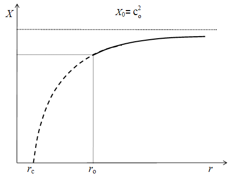 | Figure 2. Gravitational potential |
The equations (6) concern a body. The radial gradient of its inhomogeneous field causes the concave curvature of the tangential beam. Without clear physical sense or theoretical benefit, GRT ascribes this phenomenon to the equivalent space curvature. With respect to other celestial bodies, the sum of all relevant ratios mi/ri is understood in (6b). The speed of propagation at each location is determined. On the other hand, the same factors determine the reference frame for this speed. Irrespective of its physical interpretation, the potential plays the role of the medium.
9.5. Summary
Convective inductions near the bodies moving through external fields are treated. This treatment is based on the medium stratification into the vacuum and material layers. Influenced by the external fields, the material layers are respectively polarized statically. With thus formed material fields, the fields associated to them in the surroundings are moving with respect to the locally preferred frame, causing respective convective inductions, resting in the medium. Via the primary static, the final convective inductions are scaled by the fractional factors, dependent on the relative EM factors. These factors were hidden by the artificial asymmetry of respective two SI relations. By thus determined fractional factors, the current of EM wave energy is also transformed depending on the medium motion. A moving body carries by itself material fractions of energy, temporarily accumulated in it. Depending on the direction of the motion – with respect to the propagation, the correction consists of the spatial vector components. Formerly used Fresnel’s factor is reduced to one of the two fractional factors only at exclusively dielectric or magnetic media. If any of the medium features cannot be neglected, both these factors must be used separately. The application of the relativistic correction in the case of moving media does not deserve a serious attention.There is the question of possible motion of the referent vacuum medium, so far used as the reference frame. With respect to Mach’s principle, the local frame is connected to a dominant mass or its gravitational potential, as the moving medium. If, however, there exist the other, sufficiently big and near celestial bodies, with distinct motions from the predominant body, their contributions must be fractionally taken into account. The similar procedure as at the motion of the material – with respect to vacuum media, the mutual motion of various vacuum layers, or respective bodies, are to be treated. The fractions thus depend on the particular potentials and distances, in the form mi/ri, instead of the square of the radii, concerning the fields.
10. EM Induction
With respect to possible rest, motion and acceleration of the charges, the induction may be called static, kinetic or dynamic. However, this is neither ever in accord with the motion of elementary particles, nor this motion ever accords with the use of respective Maxwell’s equations. This is also related with vortical or non-vortical form of induction. In general, at motion of electricity the induction is kinetic, but at acceleration or magnet motion – dynamic.
10.1. Introduction
Though being a fundamental effect, EM induction is not elaborated in general. The inconsistent classifications of its various types contribute to its insufficient elaboration and non-systematic consideration. Noticed in the resting circuits, it is called as static induction. Related with variable currents, as the accelerated electricity, this is the dynamic physical process, treated by temporal derivatives of EM quantities. Only the cases of the affection of present bodies by external fields represent the static inductions.The induction caused by mutual motion of a conductor and magnetic field was called as dynamic induction. With respect to the motion itself, this is the kinetic phenomenon. Its algebraic expression v' × B, where v' = v – U the mutual conductor-field speed, is substituted by kinetic, equivalent to temporal field derivatives (v' · ∇B = ∂tB) – in respective Maxwell’s equation. At motion along the field homogeneity, transverse to its gradient, the kinetic derivative annuls. The differential treatment is thus called in question.
10.2. Traditional Treatment
Let a measuring instrument be connected by the sliding contacts to a horizontal conducting bar, all – in the vertical magnetic field. Each of these three partakers can be moved, lonely or with another of them, in relation to remaining two or one. The results of all the six combinations are known: the induced voltage has the value e = Blv – or zero, where l is the width of the bar, orthogonal to the field and motion. More or less convincing separate explanations of the six particular combinations can be met.Instead of the subjective orientation, with respect to an observer, all the three partakers are usually treated equally, and observed from outside. The induction depends on the mutual motion (v' = v – U) – of a circuit part (the bar or instrument) and magnetic field, in relation to the resting part. With respect to the same effective length (l) of the two parts, the equivalent induced field may be introduced: E = e/l = Bv'. Owing to their opposite circular orientation, the final induction is their difference: e = e1 – e2. It just accords to the difference of respective vector fields: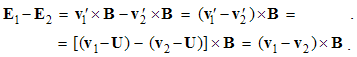 | (10.1a) |
Here v1 is the bar speed, v2 – that of instrument, and U – of the magnetic field. In principle, this equation explains the general result. Apart from the six combinations, it includes the common motion or rest of all the three partakers. The induction annuls at the motion of the full circuit relative to magnetic field, or vice versa. The consideration started and is finally reduces to the motion of a circuit part with respect to the magnetic field and the circuit remainder. In the case of the inhomogeneous magnetic field, as on the Fig. 3, its local integration along the circuit is needed. This is reduced to the famous Faraday’s law: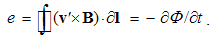 | (10.1b) |
The negative sign expresses the reactive inductive effect. Here Φ is magnetic flux embraced by the electric circuit. It is varied owing to the integral relative speed of the circuit and the present magnetic field. Due to its inapplicability to the Fig. 4, the full induction must be divided into its various special cases, presented on the Fig. 3.
10.3. Kinetic Induction
According to E = v × B, the relevant speed and induced electric, are orthogonal to the magnetic fields. The common surfaces of E&v also contain the vector A, as the vortical field, defined by B = ∇ × A . The non-vortical gradient (G) of the fields A & B, located on the same surfaces, forms the rectangular trinity with them. Let us resolve the motion and induction in the components along the vectors A & G. The motion along one causes the induction along the other of them, just in respective geometrical forms. The two cases are presented on the Fig. 3. Irrespective of its form, the induction causes closed current in the circuits. It is located by the active parts of these two circuits, moving with respect to the circuit remainder and current carrying conductor, as the carrier of magnetic field. The longitudinal motion of transverse conductor, and vice versa, causes the induction along the moving conductor.A line current (I) is producing the circular magnetic field: H = I/2πρ, where ρ is the cylindrical radius. Apart from the longitudinal induction e = Blv, the transverse one demands the integration of the inhomogeneous magnetic field along cylindrical radius or the object conductor.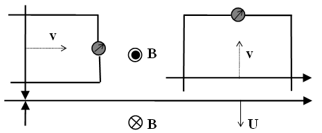 | Figure 3. Kinetic and dynamic inductions |
Not taking into account the vector A direction, algebraic treatment did not distinguish the vortical and non-vortical inductions. By the orientation to the direction of this vector, let us consider the differential treatment. Div & curl applied to E = v × B give the following two forms: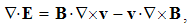 | (10.2) |
 | (10.3) |
They are reduced in particular situations. At rectilinear motion of rigid conductors, spatial speed derivatives annul, as well as divergence of magnetic field – in (3). Both forms are thus reduced to their last terms: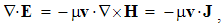 | (10.4) |
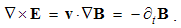 | (10.5) |
In the usual case, parallel conductor moves transversely, along the field gradient. Due to the two orthogonal vector factors, the scalar product in (4) annuls. The remaining vortical induction is described by (5), just according to the relative and temporal field derivatives.The transverse conductor is moving along the vector A. Without the longitudinal gradient, the kinetic derivative (5) annuls. The remaining non-vortical induction (4) is reduced into its transverse component. The equivalent non-vortical field accords to respective electric charge, as if located on the primary current carrying conductor: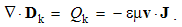 | (10.6) |
Starting from the infinity, the equivalent electric field (4) terminates on the conductor with the negative charge. Its axially symmetric electric field presents the attractive force between two parallel currents. The latter current consists of the moving electricity in the object conductor. The same formal procedure is valid for Faraday’s disc, well-known classical result (Fig. 4). The sliding contacts of the instrument terminals are connected between the center and rim of a conducting disc rotating in the front of the cylindrical magnet, around their common axis. Magnetic field is axially symmetric, without circular gradient along the speed. However, the disc speed is not homogeneous, but the linear function of the radius: v = ωr.In this case, the classical concept of variable magnetic field flux embraced by the circuit – causing the dynamic induction (e = – ∂Φ/∂t), cannot be applied. With respect to the axial field symmetry, no any flux is embraced by the circuit, and also – it is not variable at all. 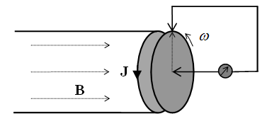 | Figure 4. Faraday’s kinetic induction |
With respect to the mentioned formal conditions, the full form (3) annuls. Apart from the latter term and its result (6), the former term of (2) must be also taken into account. The former field terminals (6) – on the apparent negative charge, are thus supplemented by the positive charge – on the disc, as the sources of the radial kinetic field: | (10.7) |
In the value 2Bω, this charge is evenly distributed about the full disc volume. The equivalent radial field terminates at the negative polarity, on the magnet cover, as the domain of the implicit magnetization current (J).
10.4. Dynamic Induction
Transverse motion of the carrying conductor displaces the radial gradient of its magnetic field, thus causing the longitudinal dynamic induction, Fig. 3. It is opposite to the kinetic induction caused by the motion of the parallel object conductor. Unlike these two vortical inductions, obeying the principle of relativity, the transverse induction, caused by the longitudinal object motion, disobeys this principle. The longitudinal motion of the carrying conductor does not influence the current in the object conductor.These conclusions are also confirmed on the Fig. 4. The magnet rotating relative to the disc does not produce any induction. Just equivalently to the common rotation of the magnet and disc, the two contacts may be connected to the magnet directly. Its conducting body takes over the former role of the disc, with the same radial induction. The differential treatments of the inductions are similarly resolved. The field derivative (8a) consists of its kinetic and dynamic components. However, the equivalent charge (8b) has only its kinetic component. | (10.8) |
Convective variation of the moving field is opposite to the field gradient and relative variations.The induction in resting conductors can be reduced to the convective effect. The increasing current causes respective growth and radial expansion of magnetic field, With respect to the equation E = B × U, this process produces the axial induction opposite to the current. At decreasing current and field, magnetic energy is returning to the conductor, with the induction – in the current direction. With respect to the transverse field motion, the induction is vortical.
10.5. Summary
The resting situation, uniform motion and acceleration of the phenomenal macro-objects are not ever in accord with respective classification into the static, kinetic and dynamic processes, respectively. The static phenomenon in a resting circuit is ascribed to the dynamic process of acceleration of the running electricity along the conductor. The uniform motion of a magnet along the field gradient also causes the dynamic induction, similarly as the accelerated motion of electricity. The induction in the moving object conductor, irrespective of its form, is the kinetic effect.Though the consistent classification of the phenomena does not give the final explanations of the processes, the application of the differential forms (2) & (3) to the kinetic induction reduced them to Maxwell’s equations. The two forms of induction and respective motion are oriented along the vector A or its transverse gradient. The general results are thus applied to a few technical situations. The local and convective inductions are finally united in interpretation, by the algebraic and differential treatments.Apart from the relativity principle, subjective orientation in relation to the arbitrary subjective observers is especially overcome. All the speeds are determined in a frame locally preferred, connected to the gravitational potential, as the medium. Refuting the artificial relativistic unification, the longitudinal induction is resolved into its two components, resulted from separate motions of the magnet and conductor. The effective transverse induction in fact represents the kinetic interaction of the two parallel currents, usually ascribed to their magnetic fields. The formal complications imposed by modern physics are here successfully overcome. The use of GRT at Faraday’s rotational experiments is also fully artificial and practically excessive. The same theory explains the forces affecting electric currents in magnetic fields. Instead of the transverse motion of the conductor with its free electricity, the electricity is moving longitudinally, thus causing the transverse induced force. Via its magnetic field, it tends to the same direction of the currents, followed by their attraction. If the conductor were stretched through the domains of the opposite magnetic field courses, it would be affected by the torque directing its current along the vector A. On the other hand, the same effect is manifest as the centripetal force keeping a free moving charge on the circular path around a tube of the present magnetic field, in the opposite course of the vector A. These two effects are the bases of the para- and diamagnetisms, respectively.
11. Complementarities
The application of differential operators to the algebraic equations gives the complex differential forms, here finally reduced to respective Maxwell’s equations. On the other hand, the substitution of the classical field transformations into Maxwell’s set gives the hybrid equations further turned into the starting set, with the transformed fields and carriers, and invariant time. Implicitly negated classical invariance of Maxwell’s equations is thus reaffirmed.
11.1. Introduction
As the basic interactions, the static laws are resolved into field actions and distributions, and the partial kinetic laws are introduced directly. The distributions of the four central fields are generalized into Maxwell’s equations. In the next step, the mutual comparison of the dissimilar fields around moving poles gives convective algebraic equations. On the other hand, the substitution of the kinetic – by static forces, relates EM fields with moving objects. The combination of the algebraic and differential equations gives the hybrid set. There arises the question of the mutual relations in this diversified family of the equations.Spatial derivatives of the algebraic field relations would give respective relations of the field derivatives. Though already obtained by some generalization of the kinetic field distributions, Maxwell’s curl-equations relate the existence of one – by the variation of the other fields, instead of their motion – in the convective equations. However, div & curl operators applied to the algebraic pair give the differential forms, formally wider than Maxwell’s equations are. Their reduction to Maxwell’s set demands zero spatial derivatives of all speeds: of the moving fields – in the convective, and of their objects – in the relative processes.Therefore, the reduction of the convective differential forms in fact understands the two rigid, stably oriented and uniformly moving EM fields. Though for arbitrary macro- fields these conditions seem to be uncertain, in the case of the elementary fields they may be base-fully expected. The rigid fields act directly at a distance, without any temporal delays. In common with their carriers, they form the stable gyroscopes. Superposition of the elementary fields gives the final effects, obeying the above conditions. The reduction of the relative forms is conventional, restricting to the rigid or punctual moving objects or instruments.
11.2. Div-equations
The motion of one EM field is producing the other of them, in accord with the two convective equations: | (11.1) |
Div applied to them gives respective differential forms, separating the non-vortical induced fields: | (11.2a) |
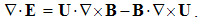 | (11.2b) |
The moving fields behave as the rigid structures, stably oriented in space. Spatial derivatives of their speeds annul, a little reducing the two above general forms: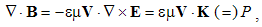 | (11.3a) |
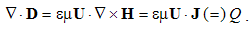 | (11.3b) |
Scalar product of the field speed and its curl expresses the axial motion of its vortices, consisting of the field line contours. They would give respective EM charges. Let us further consider the available possibilities.The vortical moving fields, consisting of the circular fluxes, are not directly connected to their moving carriers. Their motion seems to be conditioned by their own internal tensions. With respect to their circular form, such radial tensions may be expected. As such, they would cause the expansion or contraction of the field flux. Without the axial field motion, the non-vortical inductions (3) are impossible. Therefore, the convective relations, at least – in 3D space, cannot give respective two charges. The production of the quantum electricity demands an additional dimension. The axial motion of magnetic vortices along the temporal axis may possibly produce this electricity.
11.3. Curl-equations
Curl applied to (1) separates the vortical components of the two fields. Thus obtained differential forms are to be reduced to respective Maxwell’s equations: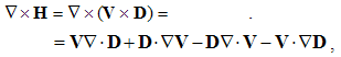 | (11.4a) |
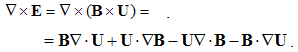 | (11.4b) |
Missing spatial derivatives of the field speeds, the right sides of these forms reduce to two terms each: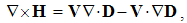 | (11.5a) |
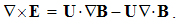 | (11.5b) |
The former term of (5a) obviously represents the causing current of the magnetic field, at left: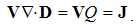 | (11.6) |
The moving charge, forming this current, is the carrier of electric field. Though compensated by the opposite polarity – in the neutral conductors, the moving electric, produces magnetic field in the domain. With respect to the vortical magnetic field, the latter term of (5b) annuls.The remaining terms, the latter in (5a) and former in (5b), represent the convective field derivatives. In accord with the opposite vector orders – in the cross products (1), these derivatives are of the opposite signs: | (11.7) |
The convective variation is opposite to the field gradient. These results give Maxwell’s curl-equations:  | (11.8) |
With incomplete div-pair, the set of Maxwell’s equations is derived from the convective pair. Obviously, this is not the strict deductive derivation. The derivation of a div-pair relies on one curl-equation, and vice versa. In any case, this procedure points to the mutual harmony of these two sets. Instead of equivalence, this is at least their complementarity. The algebraic pair relates horizontally the two fields, as the quantities of the same rank, but the differential set vertically relates the fields with their apparent carriers.
11.4. Classical Invariance
With respect to its technical realization, a field detector represents the similar resting object – of one, and dissimilar moving object – of the other EM field. Therefore, it reacts statically on one, and kinetically on the other field. The field transformations thus present the summary interactions of the fields with united pair of the two detectors: | (11.9) |
 | (11.10) |
The pair (9) multiplied by respective constant gives (10). Each of the transformed fields consists of the similar (real) – static, and dissimilar (equivalent) – kinetic fields. In the presence of only one field, one equation is reduced to the free, and the other – to their linear terms.The two operators applied, div to the pair (10) and curl to (9), with substitution of respective Maxwell’s equations into their free terms, gives the following set: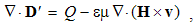 | (11.11a) |
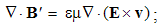 | (11.11b) |
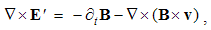 | (11.12a) |
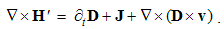 | (11.12b) |
For the simplicity, this consideration is usually restricted to uniform motion of the rigid detectors. Therefore, all the speed derivatives are here neglected: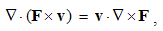 | (11.13a) |
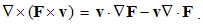 | (11.13b) |
This restriction applied to the above set gives: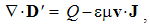 | (11.14a) |
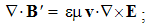 | (11.14b) |
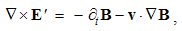 | (11.15a) |
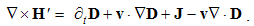 | (11.15b) |
The first equation contains charge transformation, and last – that of respective current, as the field carriers: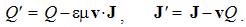 | (11.16) |
The sums of temporal and relative derivatives – in (15), transform the two displacement currents: | (11.17) |
Apparent magnetic charge (14b) is the reaction of electric field to the moving magnetic objects. It is treated as the linear term of respective charge transformation. The hybrid equations thus reduce into the standard forms: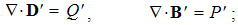 | (11.18) |
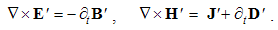 | (11.19) |
These are just Maxwell’s equations, with all transformed quantities. Apart from the fields, these are also their carriers, including displacement currents. The relative equations (9) implicitly understand all the classical kinematical relations. The classical invariance of Maxwell’s equations, implicitly called in question in SRT, is thus reaffirmed.Instead of the extensive procedure in the componential equations, or of application of the concise tensor calculus, the analogous relativistic invariance may be shown in this way, of course, with respective kinematical transformations. In fact, the invariance is the necessary, but not sufficient conditions for affirmation of the classical and/or relativistic views. In the final instance, this fact does not confirm anything, but only tries to exploit the traditional authority of Maxwell’s equations for affirmation of SRT.
11.5. Summary
The differential forms – from the convective equations – are wider than Maxwell’s set is. Their respective restriction reduces the validity of the convective pair to the rectilinear translation of the rigid EM fields, stably oriented in space. With respect to a provisory explanation, the motion coaxial with the field vortices is excluded in 3D. Though both sets origin from the same interactions, the algebraic is obtained by comparison of the static and kinetic fields, and differential – by their separate generalizations. This is manifest at the above analysis. At derivation of one, apart from respective algebraic, the other inhomogeneous differential equation is used. Instead of mutual equivalence of the equations, the complementarity of the two sets in the whole is here also affirmed. The differential set defines the assumed carriers by the phenomenal fields, and algebraic pair directly mutually relates the two fields.Field transformations applied to Maxwell’s set already gave hybrid equations. With consistent transformation of the variant quantities, their analysis again gives Maxwell’s set, with all the transformed quantities. The relative EM inductions are in the essence of this procedure. The classical invariance of Maxwell’s set is thus reaffirmed. Not only that this result does not deny similar relativistic invariance, but is the real basis for it. By complementary deformations of the transverse EM fields with longitudinal and temporal axes, all the formal relations, including Maxwell’s set, are conserved. The relativistic invariance is not the reason for negation in advance of the classical one.The field transformations are introduced as the necessary condition of invariance of Maxwell’s equations. However, this condition is not sufficient. Apart from transformation of the position, and of EM fields – as its formal consequence, electricity and current – as the field carriers, including both displacement currents, are to be transformed. With respect to the punctual objects, there is no restriction of the form of their motion. In the aim of simplicity, it is still restricted to uniform rectilinear motion. The same conditions are already habituated in the relativistic considerations. The invariance conditioned by the transformed quantities is known as the covariance. Assuming the invariant gravitational mass, the respective law would be unconditionally invariant.
12. Ampere’s Problem
The proper kinetic interaction – between two elementary electric currents – is considered. Instead of the resting field convectively induced, its transverse motion is taken into account. The speed of this field is determined and applied to the general case of a charge freely moving. The obtained general force is resolved and its components interpreted. In spite of the ellipsoidal field deformation, the even pressure about spherical particle surface is confirmed.
12.1. Introduction
By analogy with static law, the kinetic interaction of two elementary currents, as the segments of line currents, was investigated. Though the problem has not been resolved in general, such interaction of parallel line currents is taken as the bases for definition of the line current unit. The integral interaction of two electric circuits can be met in some text- books. Though the longitudinal force component does not obey action-reaction symmetry, its circular integral annuls, reducing the kinetic interaction to the remaining, transverse force. Of course, the general problem is thus not resolved, but only bypassed in this particular case.Elementary electric currents cannot be separated from the line conductors. Instead, there remains the consideration of the proper kinetic interaction of two moving charges, as the convection currents. Such the treatment of a moving electric dipole, as the two anti-parallel currents, is the next example. The routine procedure predicted some torque of the axial forces affecting the free moving dipole. Not only that such a torque cannot be confirmed in the practice, but it calls in question the action-reaction symmetry generally established. Namely, all physical forces, including their torques, must be balanced by the same opposite reactions.There is an inconsistency, so far copied through the text- books. The interaction of one, – by the field of the other moving charge, depends on the mutual motion of the object and field. Apart from the object motion, the field speed of the magnetic field must be thus known. No one of the two alternatives can be accepted. The resting field already gave the unacceptable torque, but its motion with commonly moving charges would annul their transverse interaction. Its transverse motion, as the only remaining possibility, finally resolves the problem, in the form of the general kinetic law, obeying all the known empirical effects.
12.2. Boundary Conditions
Electric currents consist of the convection or conduction of free, and of displacing bound electricity. All the three components produce magnetic fields in their surroundings, interacting with such other currents, according to the basic laws of the field distribution and action: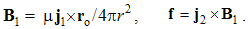 | (12.1) |
Here j1 = q1V is the carrying current, and j2 = q2v object elementary current, where r = rro is the position of the latter in relation to the former currents. The field is determined in the frame moving with its carrier, irrespective of its own motion. The law (1a) is invariant only in this reference, thus pointing to indispensable field replacement.The force (1b) depends on the object motion through the field. If, however, this field is also moving, the mutual speed of the object and field must be considered: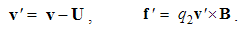 | (12.2) |
Here U is the speed of the magnetic field, distributed in space. It should be somehow determined, at least in the typical situations. At the rectilinear motion of a permanent magnet, as the carrier, this speed is homogeneous and equal to that of magnet. At a common motion of two charges, the same motion of their fields would annul the mutual speed (2a) and kinetic interaction (2b). On the other hand, the resting field would fall behind its carrier.The collision of the two unacceptable alternatives can be overcome by founded supposition of some transverse field motion. Namely, the circular form of the magnetic field flux points to its possible radial tensions, as the causes of its expansion or contraction. The moving charge and its field are thus related as a car and its wheels, moving together, but in two distinct manners. These boundary conditions are the bases for the speed determination, which would obey all the theoretical demands and empirical facts.
12.3. Field Motion
By means of the above conditions, let us determine the general kinetic force dependent on the three speeds: that of the carrier, of the object and field. The field elimination, by the substitution of (1a) into (2b), after arrangement gives the general proper kinetic interaction: | (12.3) |
The factor n = μq1q2/4πr2 simplifies all the following equations. In this sense, by substitution of the two constants, 1/ε = μc2, Coulomb’s electrostatic law turns into simple and convincing mathematical form: fs = nc2ro.The force (3) is thus resolved into the two components: axial – in direction of the motion, and radial – along the radius-vector. In the closed physical compositions, as the moving dipole is, the action and reaction of its poles must be symmetric (f2,1 =– f1,2), without any torque. In spite of the force symmetry, f(–r) =–f(r), the axial pair would form a torque on the dipole (consisting of the two charges) – in its oblique position relative to the motion.In the aim of simplicity, after substitution of (2a) into (3), we separate the two force components: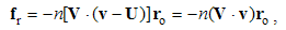 | (12.4a) |
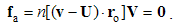 | (12.4b) |
With respect to the transverse field motion, the product VU annuls, making the radial force (4a) independent of this speed. From the similar reason, it is independent of the transverse object speed component, and represents a central interaction of two parallel currents. Its negative sign points to the attraction of the parallel, and repulsion of anti-parallel currents. The same force affects the carrying charge, by the even pressure about its spherical surface.On the other hand, the zero axial force (4b) demands zero scalar product in the brackets. With respect to the common longitudinal speed (v = V), with the assumed transverse speed U, the mentioned condition finally gives: | (12.5) |
Here θ is the polar angle, between the speed V and radius. Thus, (5b) describes the magnetic field motion around a moving charge. The function cotθ, odd with respect to the transverse plane, points to the flux expansion – in the front, and shrink – behind this plane, with the stoppage and return of its motion – in this plane. As if, these field contractions just enable the uniform particle motion.With respect to (5b), the field speed tends into infinity around the axis. There is the question of its interpretation. The final elaboration of this theory identifies magnetic field as the curl or transverse gradient of the kinetic potential. As the motion of the central static potential, this one is also in the same form. Longitudinal cross-sections of equipotential surfaces give the family of concentric circles: | (12.6) |
The transverse variation of a moving circle height (Fig. 5) equals to its negative speed multiplied by circle derivative (6b), thus confirming the result (5b).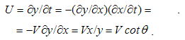 | (12.7) |
The two potentials (static & kinetic) overlap in space and move with the carrying charge. However, their transverse gradients vary in accord with the function (7). This simple illustration clearly negates a substantial essence of magnetic field, and reduces it to the formal feature of the potential. With the potential moving at a finite speed V, its transverse gradient expands at respective speed (7).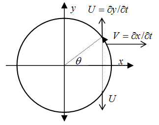 | Figure 5. Moving central potential |
12.4. General Equation
Though annulled at the equal speeds of the object and carrier, the axial force component in general must be taken into account. On the other hand, as being independent of its objects, the speed value of magnetic field around a moving charge (5b,7) is valid in general. As such, it determines the general form of the proper kinetic law.Let us resolve the forces (4) into their subcomponents, with substitution of the speed relation (5a) – into the third term of the obtained resolved axial force: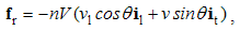 | (12.8) |
 | (12.9) |
Possible circular motion of the object charge – along the present magnetic field – would not produce any force. Its relevant speed may be thus reduced to the longitudinal and transverse components, with our observation and procedure restricted to a longitudinal plane of symmetry. The two opposite former terms (in fact introduced by the formal procedure) mutually cancel, and so the final force is reduced to the three remaining terms: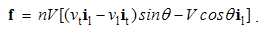 | (12.10) |
This is the general form of the proper kinetic interaction. Depending on the polar angle, the function sinθ is odd around the axis, but even – in the longitudinal sense, and vice versa – for cosθ. These facts determine the integrals of the components (10) around a carrying line conductor, as the continual sequence of elementary currents.The two former terms (10) accord to the force (1b) acting on a moving charge through the resting field: | (12.11) |
By this force, magnetic field affects the resting current carrying conductors: the former term – by the torque – onto transverse, and latter term – by the transverse force onto the longitudinal conductors. Along moving conductors, these forces cause respective relative inductions.The third component of (10), independent of the object motion, represents the longitudinal electric field. Owing to the function cosθ– longitudinally odd, this field annuls at line currents. Around a moving charge it is directed axially, towards the charge. Subtracted from the static central field, it gives the impression of the ellipsoidal field deformation. Towards the boundary speed c, the result tends to zero, with effective charge diminution in the ratio 2/3.In the common motion of two charges, at the longitudinal speed vl = v (but vt = 0), the first term (10) annuls, reducing the kinetic force to the remaining two terms: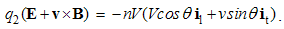 | (12.12) |
Unlike the longitudinal electric force, the transverse one, dependent on the object speed, is the magnetic interaction. These two force components taken together form Lorentz’ kinetic force, given at left. In the moving frame – connected to the carrier, with V = v, these forces form the combined central field, f = – nv2ro, producing the even pressure about the particle surface. The field speed (5b), here successfully applied, is thus also further affirmed.The force (12), as the interaction of two parallel currents, distinguishes from the radial force (4a) by the speed V – instead of v, in the axial direction. At the equal speeds, as at a moving dipole, the sum represents the central force. In a line current, the axial (odd) forces annul, with remaining integral of the radial components. This radial component, also more operative than the correct Lorentz’ force (12), is usually sufficient, as at mentioned annulment of the circular integral of the axial force, in electric circuits.
12.5. Summary
This exposition started from the classical Trouton-Noble experiment, with assumption of the transverse field motion, in the aim to explain the obtained result. Owing to needed balance of the forces and torques in the closed physical compositions – as a free dipole is, only such result can be expected. After exclusion of the rest & axial motion of the magnetic field, our assumption has no alternative. Apart from the intuitive reasons, it is confirmed by the kinematic interpretation of the moving potentials.The formal procedure of gradual derivation, with its final interpretation, gave the general form of the kinetic law (10). As such, this result confirms the two pairs of the classical results: the transverse force between parallel, and the torque between crosswise line currents; unidirectional induction – in the longitudinal, and symmetric – in transverse moving conductors. The ellipsoidal deformation of electric field and the even pressure per the particle surface represent the third pair, already announced by H. A. Lorentz. The former effect from the last pair, caused by transverse contraction of the magnetic field, was formerly introduced intuitively, without any due explanation. Without additional physical or technical arguments, SRT ascribes this effect to the increased transverse, instead of diminished axial field components. Complementarily to the deformed electric, the moving charge is also affected by the transverse magnetic forces, giving the central force, as the result.
13. EM Inertia
From the proper kinetic, dynamic interaction is derived. The mutual and proper masses, as the factors of induction or self-induction, are thus determined. The inertia of neutral bodies is reduced to self-induction of the particles in the structure. The function of mass against speed of its motion is formulated and clearly interpreted. The dynamic force is resolved into its inertial and centrifugal components, of the electric or magnetic natures, respectively.
13.1. Introduction
Though mass is adopted as the basic physical quantity, the unity of its various forms is not established. By the two Newtonian laws, of force action and gravitation, respective two masses are introduced mutually independently. With respect to the predominantly empirical origins of these two laws, their final essences and mutual relations are still not determined. In the absence of their final comprehension, the two masses are compared quantitatively in the sequence of various bodies or particles. In the frames of the reliable measuring, their proportionality in the wide quantitative range is allegedly established. However, this fact is not sufficient for their qualitative equivalence.In addition, the unity of various inertial phenomena may be also called in question, in spite of their common formal treatment. In experience and primary verbal formulation of inertia, the two conservations are observed separately: of the speed and direction of the motion. A body opposes to all the external forces by the inertial and centrifugal reactions. Though both of them are understood in the vector form of force action law, they are essentially distinct. The former force, independent of the momentary speed, transfers the energy at acceleration. As the function of speed, the latter force is not engaged in this process. Though also mutually proportional, the essences of two respective masses are not united in the mechanical frames at least. Though manifest, some formal similarities of mechanical and EM phenomena did not contribute to their unification. The same form of the static central laws is insufficient for any their relation. Apart form the two exclusive forces, the substantial distinction in polarities of electricity and mass separates them. Similar relation separates the two dynamic phenomena, inertia and induction. Though both depend on acceleration, inertia affects the accelerated body only, but induction also affects its surroundings. On the other hand, their similar resolution is not noticed. Alike the centrifugal force, respective induction is also manifest by the transverse (radial) forces affecting electric circuits.
13.2. Mutual & Proper Masses
In the aim to formulate the dynamic, we start by the two kinetic laws, basic and alternative ones: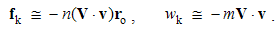 | (13.1) |
The former of them expresses the mutual kinetic force, and latter – respective energy. In the longitudinal direction, they are restricted to the equal speeds. The integration along radius of the former gave the latter law, turning the kinetic (n) into the dynamic (m = nr) factors: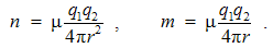 | (13.2) |
Partial derivative of the mutual kinetic energy (1b) – per mV, gives the power of its transfer, from the active force – via the carrier – to the affected object: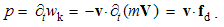 | (13.3) |
In the partial derivative, the speed v is a parameter, with the factor m dependent on the radius. The power equals to the product of the object speed and dynamic force, obtained in the form of force action law (4a), with the law of inertia as its special case (4b) – at the zero force: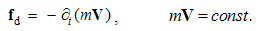 | (13.4) |
The product mV accords to linear momentum. Therefore, the factor m, as the measure of electric inertia, represents the mass, mutual (5a) or proper (5b):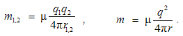 | (13.5) |
Depending on the two charges and their distance, the mutual mass determines the object reaction on the carrier acceleration, or vice versa, of course. Their interaction is mediated by the full dynamic field, as the distributed force. In the same way, this field affects in return its own carrier, depending on the proper mass. The particle radius (r) is the distance of the surface charge from its center. The smaller particles are of the greater masses, and vice versa. The classical electron radius is thus obtained.Respective phenomena are known from electric circuits as (self)-induction. In accord to the axial dynamic force, it depends on the first power of distance. At globally neutral bodies, as EM multi-poles – with qi = 0, the mutual mass fails. The self-induction of a pole, as the consequence of the associated electric field placed around it, is manifest as the mechanical inertia. Owing to the mutual cancelation of the opposite fields in the wider surroundings, the final mass is less than the sum of the separate elementary masses. This effect is well-known as the mass defect.
13.3. Mass Function
Let us compare the masses (5). The mutual mass depends on the distance of the poles, and can be changed by this distance. Their particular radii do not play any role in this mass. On the other hand, the proper mass depends on the particle radius only. There arises the question of possible variation of the latter of these two quantities.The particle radius, as the elastic charge surface, depends on the balance of the internal and external pressures on the surface. The internal pressure is determined by EM fields, or respective two forces – static and kinetic: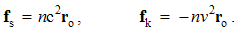 | (13.6) |
A resting particle is affected by the former positive force, along the radius. This effect reminds the gas pressure on a bloated balloon. Its explosion is prevented by the constant external pressure, similar to the atmospheric, on the balloon. With respect to the inverse function (2a), the internal forces decrease at the expansion, keeping the balance with the constant external pressure, at a certain radius. The radius and mass are thus strictly determined.The internal pressure at a moving particle is diminished by the additional kinetic forces: | (13.7) |
The factor (2a) is the function of radius, n = n(r), and g2 – of the speed. The balance with the same external pressure is thus established on the smaller radius: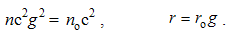 | (13.8) |
Here ro is the radius at rest, and no = n(ro) – respective factor. According to (5b), there follows: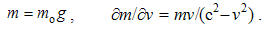 | (13.9) |
The mass function (9a) was primarily introduced by H. A. Lorentz, by the help of empirical data. Its introduction as if took into account the even pressure on the particle. From (9a) directly follows its derivative (9b).With respect to (9a), the mass of a charged particle, as well as that of a neutral body – as the aggregate, grows by the speed. At the smaller speeds at least, it is assumed in the constant value. Towards the boundary speed (c), its function (9a) rapidly grows asymptotically, tending into infinity. Simultaneously, the particle radius is gradually compressed up to zero. This fact explains the boundary speed of the acceleration, otherwise mystified in SRT.
13.4. Linear & Radial Inertias
The linear momentum consists of the three factors. Its derivative thus obtains respective three terms: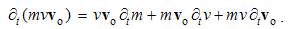 | (13.10) |
Here v is modulus, and vo – the unit vector. With respect to (4a) & (9b), the two forces are obtained: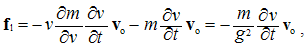 | (13.11) |
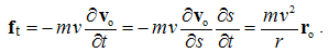 | (13.12) |
Here r is modulus, ro – the curvature direction, and s – the path taken. Owing to the variable mass, the longitudinal inertia (11) is corrected by g2. The transverse inertia (12) known as centrifugal force, tends to rectilinear motion. At motion of globally neutral bodies, these forces affect the elementary particles in their structuresAlike kinetic, the dynamic force is also resolved into its longitudinal – electric and transverse magnetic components. The phenomenal distinctions of these components are thus explained. Without mutual relations of the two fields, the two forces seemed to be the distinct phenomena. The same EM effects are easy to explain. By its own magnetic field, a current is compressed in a line conductor, but tends to expand its circuit radially. The kinetic interactions of the concentric electric circuits also resemble the centrifugal or centripetal forces. Unlike these two, the proper centrifugal forces affect the same particles themselves.
13.5. Summary
On the elastic particle model, the mass-function against speed is here confirmed. Its growth at acceleration is the consequence of the particle compression, by the additional EM fields. When the speed tends to the boundary value (c), the particle radius tends to zero, and mass – to infinity. The upper boundary speed of the particles and their sets is thus explained. The particle volume diminution up to zero calls in question a solid particle body, distinct from its fields. As the increasing quantities, mass and energy are contained in the particle field. The increased domain of the electric field just accords to these greater quantities. Apart from the (static) gravitation and (dynamic) inertia, mechanics operates by the kinetic – frictional forces. After neglecting the friction, the laws of mechanics seem to be invariant with respect to the uniform motion. However, apart from the reference of acceleration, in the force action law, there is the question of the reference of speed, in the mass function (9a). With respect to the external pressure on the particle, certain vacuum medium, as the reference frame, is understood. Just when is resting in this frame, the mass is minimal. The subjective orientation in space, speculatively assumed in SRT, must be finally refuted.The mechanical phenomena are reduced to EM processes around charged particles. There is very difficult to expect an additional basis of these phenomena, thus expecting the EM nature of matter. Though avoided in the modern physics, the reduction of matter to electrons and protons may be worth of consideration. On the other hand, with respect to the invariance of mutual mass of two interacting charges, similar invariance of gravitation, as the mutual phenomenon, may be expected. The postulated equivalence of the two masses is thus called in question. The relation of gravitation with EM phenomena remains still open.
14. EM Energy
The mutual energy of two particles is determined by the difference, and proper – by the sum of the static and kinetic components. The energies bound in EM fields are identified as respective medium disturbances. Poynting’s theorem is derived and identified as the 5D continuity equation. It also contains the algebraic expression for the energetic current. The substitution of each of the convective equations into this expression gives respective energy current, also applied in the surroundings of a moving charge.
14.1. Introduction
Being inaccessible by sensory perception, energy is very abstract physical quantity. On the other hand – in everyday life, it is a concrete notion. Not only that it is successfully produced, measured and transferred at distance, but – as any other goods – it is regularly marketed and spent. Industrial production and biological existence are based on the energy. Between its two starting, at least apparently – incompatible notions the complete development of physics may be placed. By the long sequence of the formal relations and procedures, the sensory nothing is gradually transferred into practically everything. With respect to incomplete interpretations, they are still the two irreconcilable extremes.Though intuitively very similar to linear momentum (mv), the expression for total energy (mv2) is of a distinct physical sense. Not only that their formal natures (vector & scalar) are distinct, but they are also not mutually proportional. In spite of these distinctions, each of the two quantities is conserved in the closed physical compositions. However, unlike mechanical notion of momentum, energy manifests in all physical processes, but in the various forms. More or less successfully, these forms are transformed into each other, with full mutual equivalence. Irrespective of all, the unique final essence of energy is not known.In the scientific sense, energy is a scalar physical quantity, absolutely homogeneous in 4D space. Its distribution at the structures just represents these structures. In each structural layer, a force field is closely related with respective energy, as the gradient of its density. The balance of various forces accords to the energy homogeneity. The interactions of two confronted forces are followed by energy transfer, with the motion in the course of the active force. With the dynamic force balance, a moving body accepts the energy from the active, and returns it to reactive fields. The two processes are conveniently distinguished by the opposite signs of the energy and the power of its transfer.
14.2. Bound Energy
On the various structural levels, the energy is distinctly interpreted, defined and calculated by various procedures. The alternative central laws determine the mutual energy between two moving charges, as the difference of the static and kinetic energetic components: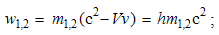 | (14.1) |
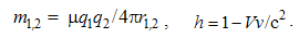 | (14.2) |
According to the mass (2a), the referent zero of both components is at infinity. In the case of common motion of the two charges (v = V), their distance and mutual mass are constant. However, the mutual energy declines by the speed, from the static value – at rest, it tends to zero – at v = c. This is the result of the two opposite components.However, the proper energy of a body seems to be of the other physical nature. Differential of the kinetic energy is expressed by the power of its transfer, equal to the product of the body speed and active force, with the force pulse equal to the linear momentum variation: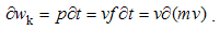 | (14.3) |
On the other hand, by a routine procedure, from the mass function (4a) – its differential (4b) is obtained: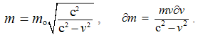 | (14.4) |
From (3) follows left, and from (4b) – right equality (5):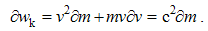 | (14.5) |
Assuming the constant mass, the former middle term annuls. The simple integration of the latter term gives the incomplete energy, wk = mv2/2, wrongly ascribed to the motion of the invariant value of mass (mo).Instead, the trivial integral of the external equality (5), from the resting mass (mo) – up to its value (m) – in motion, gives well-known Einstein’s result: | (14.6) |
The kinetic energy just accords to the difference of the two values of mass. The final substitution of mass identifies the electrical energy between the two radii.This result is in harmony with Maxwell’s interpretation of the energy accumulated in respective force fields. It is manifest and expressed by these two fields: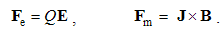 | (14.7) |
As the gradients of respective energy densities, these two fields affect their respective objects. The potential energy equals to the work done at the object displacements through each of respective two EM force fields: | (14.8a) |
 | (14.8b) |
Unlike the infinity – at central laws, the zero disturbances – at regular media, are here the references.The integrals of rational fields give the energy densities at the media disturbed by respective force fields: | (14.9) |
With respect to collinear fields in the pairs, the vectors are substituted by the scalars. The application of (9a) to the central electric field of a punctual charge gives a half of the energy (6), obtained from the central laws, without factor 1/2. These two may be the components of manifest energy, without their needed but hidden halves.On the other hand, the total fields resolved stratify these energies between respective structural layers: | (14.10a) |
 | (14.10b) |
In fact, each of the energies is distributed between the vacuum and respective material structural layer. This result is already used in lesson 9, at the consideration of moving media. As will be shown (15), the vacuum layer plays the role of the energy transferor through space.
14.3. Continuity Equation
At the motion of the carriers and their fields, respective energies cannot stay at rest. The needed analysis starts by the two Maxwell’s curl-equations:  | (14.11) |
The former of these equations multiplied by the field H, and latter – by E, with subtraction of the latter from former results, gives the following equation: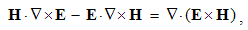 | (14.12a) |
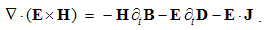 | (14.12b) |
The two left terms in (a) give the divergence of the cross- product, equal to the sum of the three dot-products (b). The former two of these three terms express the variable energy density, and third – the power of its dissipation: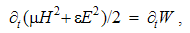 | (14.13a) |
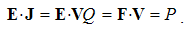 | (14.13b) |
The equality (a) presents the temporal variation of energy density, and (b) – the speed of its transfer. The equation (12b) thus turns into Poynting’s theorem: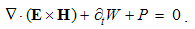 | (14.14) |
This is 5D continuity equation of EM energy. Its three terms concern the main subspaces in 5D: 3D space with the temporal and structural axes. The first of these terms just operates by the spatial energetic current: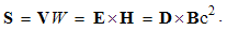 | (14.15) |
Einstein’s equation by EM fields is added. With the two vacuum fields, forming the current, the total fields accord to the current of mass, or equivalent momentum.
14.4. Energy Flows
The substitution of each of the two convective equations (11.1) into (15) gives the two energetic currents, related with motion of respective EM fields: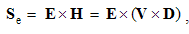 | (14.16a) |
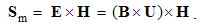 | (14.16b) |
Depending on the moving fields, the two processes may be mutually related or practically independent. The former of them concerns moving electric, and latter – magnetic fields. The further formal elaboration gives: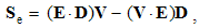 | (14.17a) |
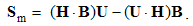 | (14.17b) |
At the interaction of the moving and induced fields, the current is determined by the moving field and its speed. The former terms represent the energies running at the field speeds. The moving densities depend neither – on the field speeds nor on respective inductions.The double values of the mainstream moving densities, with respect to that in the medium, point to the other their halves, un-manifest directly. The invariant densities point to the expanded domain (on account of the particle volume) as the only possibility of the energy growth. The latter terms express the accessory flows, between the carriers and the medium, along the fields. The dot-products influence only their intensities. Irrespective of the carrier type or polarity, the energy flows from the medium towards the carrier – in the front, and in the same amount is returned to the medium, behind the moving carrier. Around a moving charge, the energies (17) are summed. The latter term of (17b) annuls, due to perpendicular factors. The remaining three terms finally give: 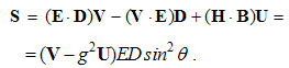 | (14.18) |
The full current is resolved into components. The latter of them can be conveniently accommodated: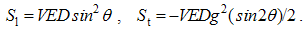 | (14.19) |
The known speed relation V cosθ = U sinθ, substituted into the latter term, gives the product VED, enabling the comparison. Positive in the motion course, the longitudinal component is mainly located around the transverse plane of symmetry. This is the alternative interpretation of the wave or photon associated to the moving particle.On the other hand, the transverse component – in (18), proportional and opposite of the field motion, depends on the factor g2. Approaching the speed c, it tends to zero. The expression (19b) determines its angular location, about the cones of 45o & 135o. Being opposite on the two sides, it does not influence the moving energy amount.
14.5. Summary
The energies around moving charged particles, mutual & proper, are expressed in the form of Einstein’s equations. The former is obtained as the difference, and latter – as the sum of the static and kinetic components. Approaching the speed c, the mutual energy tends to zero, and proper – into infinity. Instead of their complementarity, the former trend results from the cancelation of the opposite forces, and latter – from the particle compression. On the other hand, with respect to the inverse function (4a), the mutual energy also declines by the increasing distance. Simultaneously, the common mass defect is thus avoided.The Poynting’s 5D continuity equation (14) identifies the term E × H as the energetic current. Its application to a moving electric charge gives the moving density in the full value ED. On the other hand, the way of derivation of the continuity equation also points to an additional quandary. Irrespective to the moving EM field, (13a) understands both these energies, electric and magnetic. They result from the simultaneous application of both Maxwell’s curl-equations, as at a closed causal process. In the final instance, alike the closed EM fields in 5D space, the closed essence of all the causal physical processes may be expected.
15. EM Waves
Differential and algebraic treatments of EM waves are presented and compared, with the harmonic supplement or overlap of their results. The medium stratification enables energetic interpretation of the wave propagation. Vacuum layer is identified as the wave conductor, which really transfers the wave energy. Accumulating temporarily a fraction of energy, material layers increase its density and slow down the propagation. The separate effective speeds of the two EM fields are also identified.
15.1. Introduction
In the general approach to elementary structure, let us consider a linear rotator, as its typical element. It consists of a massive body m, connected by elastic tie to the center of rotation. Let the tie extension be proportional to the applied centrifugal force: r = ef, where e expresses the tie elasticity. For each tangential speed, v = r, the balance of the two forces (1a) is kept. Its direct division by the product mr finally gives the invariant angular speed (1b):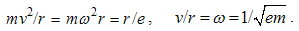 | (15.1) |
With proportional variation of the speed and radius, the angular speed depends on the two factors (e & m) only. The multiplication of (1a) by r/2 points to the equal amounts of kinetic and potential energies of the rotator: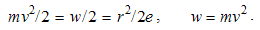 | (15.2) |
The full energy is in the form of Einstein’s equation. The interpretation of the two quantities depends on the observed physical processes. In the aim of their general interpretation, let us observe a medium formed of multiple such rotators, as the basic structural elements. The mean molecular energy determines the medium temperature: w = m<v2> = kT. The average speed (<v> = c) just expresses the thermal medium activity. The substitution into (2b) gives: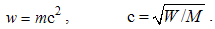 | (15.3) |
Volume derivatives turn the discrete quantities of mass and energy into their densities, as respective fields. The typical expression for the speed of propagation (3b) is thus obtained. At various waves and media, there are respective interpretations of the two densities. In principle, the value M accords to the total energy, and W – to its free component, propagating through the transferring layer. Their difference, accumulated in the cruder medium, temporarily rests. There follows respective analysis of EM waves.
15.2. Wave Equation
Approaching a conductor, EM wave induces the reactive currents in it. Thus obtained opposite fields constitute the reflected wave. The undisturbed propagation is thus reduced to the non-conducting media. At dielectric media, without free electricity and respective current, the free terms of the two inhomogeneous Maxwell’s equations annul. Apart from the div-pair, pointing to the vortical field forms, the further analysis is thus reduced to the curl-pair: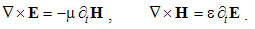 | (15.4) |
Curl applied to one, and ∂t – to the other of them, with elimination of one field, the other forms the equality: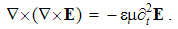 | (15.5) |
The left double product turns into the two terms: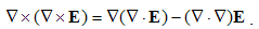 | (15.6) |
Due to the vortical field, the former term annuls, thus turning (5) into the following typical form: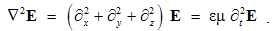 | (15.7) |
By its form, this is wave equation. The product of the two constants determines the speed of propagation: c2 = 1/εμ. There is obvious its trivial solution: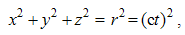 | (15.8) |
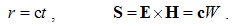 | (15.9) |
It points to the radial EM wave, propagating at speed c. With respect to the energetic current (S), both EM fields are perpendicular to the direction of wave propagation, i.e. the two fields just determine the wave front and direction of propagation. Irrespective of its kinematical sense, (9a) gives the effective speed of propagation, dependent on the two medium features: c2 = 1/εμ. The opposite solution of the equation (8a), introduced by additional derivatives of the starting equations (4), is not taken into account.Just on these bases, Maxwell predicted EM waves and their speed of propagation. The light is reduced to the same nature. EM waves obtained by H. Hertz were the decisive condition of the final acceptance of Maxwell’s EM theory. Though this acceptance was late at least for 20 years, it was too early – with respect to the incompletely elaborated EM theory. Starting by the intensive practical applications, its elaboration is left for the future times. Its algebraic aspects, merrily here elaborated, are especially neglected. Maxwell’s equations are usually treated as the postulates, confirmed by the long time of their successful application.
15.3. Moving Fields
Let us now consider possible further contributions of the algebraic equations to the wave theory. In this aim, we start by the two convective algebraic equations: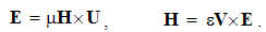 | (15.10) |
One of the two fields is easily eliminated. Owing to the closed causal loop of the wave propagation, the same field figures on both sides of the obtained equation: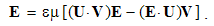 | (15.11) |
In the case of both transverse fields (TEM) at least, the latter term annuls, thus giving the identity: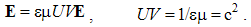 | (15.12) |
This is the pandanus of the wave equation. Its result (12b) points to possibly different speeds of the two EM fields in the same wave, with the speed of the propagation – as their geometric average. With some imagination, this result can be also obtained from Maxwell’s equations.Unlike TEM waves, one field usually has its longitudinal component. If this were electric field, the wave is of TM type. The latter term (11) is then taken into account. At least in free space, this effect is manifest by transverse expansion of the wave beam. Its consideration, however, exceeds the frames of this fundamental theory.The total fields are collinear with vacuum components. The ratio of the two collinear currents of mass and energy equals to the product of the two EM constants: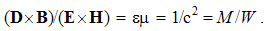 | (15.13) |
This result is already announced in the general approach (3b). With respect to the ratio of the total and vacuum fields, this is the ratio of the total energy in the full medium and its vacuum fraction. Let us consider the roles of these two energies and of their difference as well.
15.4. Energy Propagation
The energy transfer is expressed by the current S. Each convective equation (10), substituted into (9), with some formal arrangement, gives respective current: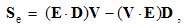 | (15.14a) |
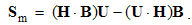 | (15.14b) |
In the cases of TE or TM waves, the latter terms concern some transverse expansion of the wave beam. In the ideal TEM wave, these terms annul, and the equal former terms express the same energetic current: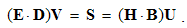 | (15.15) |
In the similar way as at linear rotator, the force balance in the vacuum component of the wave fields, independently of the two material layers, is equivalent to the equality of the electric and magnetic wave energies: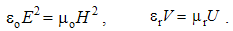 | (15.16) |
The former equality relates the two vacuum fields in EM wave. In NS units, these two fields are numerically equal. Therefore, (16a) substituted into (15) gives (16b), as the additional field speed relation. With respect to their product (12b), they can be finally determined. The elimination of one of them gives the other, and vice versa: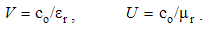 | (15.17) |
Each of them is reciprocal to respective relative factor. At vacuum, with both unit factors, both equal to co. Their product (12b) gives the refraction factor (n):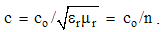 | (15.18) |
It represents the speed ratio of the same wave at vacuum and matter. The same ratio is announced by (13), but it is further emphasized by the two field speeds.The double equality (15) determines the energy current, as the arithmetic average of the two expressions on its two sides. The effective speeds (17) substituted into this current explain the process of the energy transfer: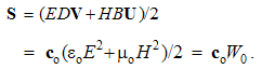 | (15.19) |
The vacuum layer only, as the basic medium, transfers the wave energy. The material layers temporarily absorb respective fractions of the full wave energy, proportionally decreasing the speed of wave propagation.Various factors in the structure, from the inert movable charges – up to the non-linearity of their mutual interactions, relate at least one of the two constants, and so – the speed of wave propagation, with its own frequency. This dependence causes the different phase delays of its various components, and so – the temporal dispersion of complex signals on the path. With respect to the factor n, the beam refracted on the boundary of two various media enables angular dispersion and obvious analyzing of the complex signals. With accumulation of the fraction of wave energy in the matter, these layers as if narrow the vacuum medium, as the wave transferor, thus decreasing the passing ability of the free space. The indispensable conservation of the energetic current on the path of propagation points to the wave speeds being above the value co. There appears that this speed also depends on the same refraction factor: | (15.20) |
The product of the external two (20a) gives the square of the middle term, expressed by (20b). The vacuum speed is the geometric average of the new wave and effective speeds. The latter speed expresses the real transfer.
15.5. Summary
Complementary analyses of the differential and algebraic equations enable multilateral explication of the process of wave propagation. Some results are thus obtained, as the different effective speeds of the two fields through material media. The separate roles of particular medium layers are determined. Among the three non-conducting layers, only vacuum, as the basic medium, transfers the wave energy. The resting portion, accumulated in the matter, increases the local energy density and decreases the speed of propagation – in the ratio n. The last effect only was known.Instead of the two fields, the treatment of EM waves may be founded on the two potentials: scalar and vector. The consideration would be analogous to that of a compressible fluid, with the pressure and linear momentum density. This analogy is used in electric circuits, operating by the fluid of free electrons. The pressure is expressed by the voltage, as the difference of the static potentials. There is expected the simpler operation with the four components of the potential, instead of six – of respective fields. In the final instance, the potentials more directly than fields express the final essence of EM phenomena. However, some advantages of the usual treatment, as the energetic current – in the form of the cross-product of the two fields, would be lost.Though EM waves are widely used, a satisfactory theory of radiation is not formulated so far. The concept of delayed potentials in advance understands the expansion, without a clear causal explanation and the energetic transfer. Each variation of the speed or direction of the charge motion is expected to radiate some energy. However, a direct current in electric circuit, irrespective of the circular motion, does not radiate at all. Moreover, which energy would be radiate from a charge accelerated by external forces? With respect to the invariant energy density around the moving charge, only the energy accumulated on account of its diminished volume can be released at its deceleration.
16. Field Transformations
The complete field transformations are based on the basic algebraic equations. The sums of moving fields and similar kinetic inductions form the primary transformations. As the interactions of the convective and relative effects, square corrections are obtained, by three in each transformation, in accord to respective terms of the proper kinetic induction. Added to the primarily transformed fields, they form the secondary field transformations, also reduced to the same mathematical form of the primary ones.
16.1. Introduction
The three main kinematical quantities (position, speed & acceleration) depend on the reference frame used. Thus the speed (v) of a moving frame changes the positions (R) and speeds (V) of the objects and their fields:  | (16.1) |
These two equations are well-known as the classical transformations of the two kinematical quantities, from a comparative (R, V) – into the moving (R', V') frames. The mutual motion at the speed v is performed for the time t, starting from the common position of the two frames. The difference (1b) represents the mutual speed of the observed objects and their observers. Apart from the absolute cosmic time, T' = T – started at the big bang, all the times, started from other instants, are invariant irrespective of a particular object, its motion and reference frame.Instead, respective two relativistic relations are imposed. Their roots and procedures of their derivation will be soon presented. There are now their formal shapes: | (16.2) |
These two equations are assumed arbitrarily, without real empirical basis or theoretical interpretation. As if borrowed from the mass function (13.9a), the factor g2 = 1 – (v/c)2, thus dependent on the frame speed, tends to zero at v = c, and the two quantities (2) strive into infinity. At small speeds, the factor g nearly equals to unit, and so (2a) turns into (1a). However, the time (2b) further remains somehow transformed. Apart from the frame motion, it would be also dependent on the object position (R) – in the arbitrary comparative frame. This formal inconsistency was overlooked for more than a century of SRT.
16.2. Primary & Secondary Equations
The field transformations are based on the basic algebraic relations, convective and relative ones: | (16.3) |
 | (16.4) |
Apart from the speeds of the electric (V) and magnetic (U) fields (3), the equations (4) operate by the speed v – of the moving frame, connected to the measuring instruments. The summation of nominally similar fields, given and induced, gives the primary field transformations: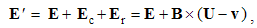 | (16.5a) |
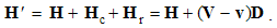 | (16.5b) |
Apart from the given fields in the free terms, the moving detector also registers the mutual kinetic inductions, in the additional terms, as the linear functions of speeds.The effects of separate motion of the two fields and their detector, as the mutual kinetic interactions, are added to the given fields. Apart from relative inductions in thus induced fields, the possible motion of these fields is not taken into account. With respect to these additional effects, the proper kinetic inductions must be added. They are obtained from, respectively applied, basic algebraic equations, and as such added to the primarily transformed fields: | (16.6a) |
 | (16.6b) |
These are the secondary field transformations, applied to the primarily transformed fields (5). They are in the same mathematical form of the primary transformations. All the additional terms will be separately determined.
16.3. Secondary Corrections
At first, we will take into account the relative inductions in the additional fields from (5), being convectively induced. Respective application of the relative equations gives the relative-convective corrections: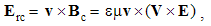 | (16.7a) |
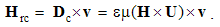 | (16.7b) |
The resolved double products explicate these equations, turning them into the symmetric forms: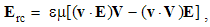 | (16.8a) |
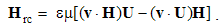 | (16.8b) |
Alike the proper kinetic interaction (12.3), each of these corrections is thus resolved into the two, mutually oblique, vector components. The former of them is directed along field motion, and latter – along the field itself.Let us resolve the detector speed with respect to the field motion. In the case of its transverse motion, the latter dot- products annul. The equations thus reduce to the remaining former terms, giving the longitudinal components of the two relative-convective corrections: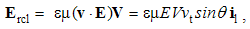 | (16.9a) |
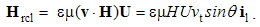 | (16.9b) |
The polar angle is determined between the field speed and the moving field itself. In the case of the electric field (9a), with n = εμq2E, the correction accords to the first term of the proper kinetic interaction (12.10).At longitudinal object speeds, the new resolution in (8) – of the moving fields with respect to their speeds, are needed. Concerning the longitudinal fields, with the three collinear vectors, the former and latter terms cancel each other. At the transverse moving fields, however, the former terms annul, reducing the equations into the latter terms, as the transverse relative-convective corrections: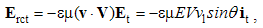 | (16.10a) |
 | (16.10b) |
The electric field correction (10a) accords to the second term of (12.10). The relative-convective corrections – (9) and 10) – result from the detector motion. Therefore, they represent the mutual kinetic interactions.With respect to the motion of convectively induced fields, respective inductions should to be also determined. They are obtained by mutual substitutions of the two convective equations (3) – each into the other: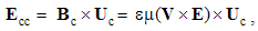 | (16.11a) |
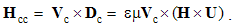 | (16.11b) |
The motion of the induced magnetic, gives the electric correction, and vice versa. They are also arranged: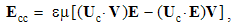 | (16.12a) |
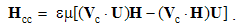 | (16.12b) |
Let us repeat the speed relation of the two related fields. The analogous relation (b) is here added: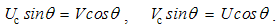 | (16.13) |
With respect to transverse direction of the induced field speeds, these equations turn into the vector form: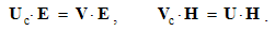 | (16.14) |
The dot-products take into account the field components collinear to the speeds, what is just expressed by the sin & cos of the polar angle. The products of the same field by two perpendicular speeds just point to the power of the energy transfer between thus related fields.The two vector equations (14) show that the ratios of the moving field components also determine the motions of the two convectively induced fields. Therefore, the motion of the latter, demands the longitudinal components of former fields. All non-vortical fields, and the vortical ones moving in their field line planes, have the needed longitudinal field components. In all these cases, the former terms (12), with the pairs of perpendicular speeds annul, and the corrections reduce to the latter terms. By substitution of (14), they turn into the following final forms: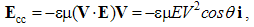 | (16.15a) |
 | (16.15b) |
Independent of their objects, these are the proper kinetic inductions. Thus subtracted from the moving fields, they diminish their longitudinal components, up to zero – at the speed c. The dissimilar convective fields tend to the values of the transverse moving components, forming by them associated waves. Thus the field Ecc in (15a) accords to the third term of the proper kinetic force (12.10).
16.4. Special Relativity
Not taking into account any motion of the convectively induced fields, with additional restriction to the common field speed collinear with that of the detector, the defective field transformations were obtained: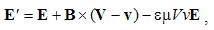 | (16.16a) |
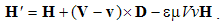 | (16.16b) |
With respect to the cross-products, the field components transverse to the motion are understood. The transverse relative corrections (10) only are thus added to the primary fields (5). Convenient term groupings give: | (16.17) |
The division by the factor h = 1 – εμVv turns these two equations into the wanted forms (5,6): | (16.18) |
The additional artificial transformations of the primed fields, in the form F" = F'/h, and also of the mutual speed of the fields and their detector, are understood: 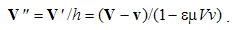 | (16.19) |
This is the relativistic speed transformation. In the case of EM wave, its speed substituted gives the alluring result: c" = c. Although practically impossible and theoretically inconceivable, it will be related with the postulated equality of all the inertial frames at least. Its apparent empirical confirmation concerns Earth, as the predominant mass, and cannot be generalized to any other frames.At the resting fields – the corrections annul, and the full transformations turn into the classical forms: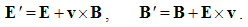 | (16.20) |
Only the detector speed remains. The formal inversion gives the inverse field transformations: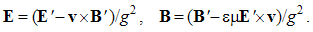 | (16.21) |
Here g2 = 1 − εμv2 is the set determinant. This factor calls in question the postulated frame equivalence. In fact, one of them, related to the medium, is preferential.For the sake of the pleasurable frame equivalence, the medium is arbitrarily denied and excluded. This is carried out by the inconsistent redistribution of the set determinant, by g–1 – in the inverse and direct sets: | (16.22) |
Their mutual inversion is saved. However, the additional transformation (F" = F'/g) – of the transverse fields, calls in question Maxwell’s equations, as their distributions. Due to their authority, their form is saved by the radical assumption. Inverse transformations of the longitudinal and temporal axes compensate the disturbed equations: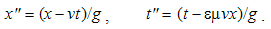 | (16.23) |
The same factor g, from the mass-function (13.9a), is not anyhow related with these formal procedures and respective views. By mutual division of these equations, the common field motion (V = x/t) is taken into account, thus returning to the transformation (19). The formal causal relation of the two relativistic postulates is thus established.
16.5. Summary
The addition of the secondary corrections – in the forms before their resolution, relative (7) and convective (11) – to the primary fields (5), gives their secondary transformations (6). With respect to the primary equations (5) as the linear functions of speed, the corrections are the square functions, with the typical term: εμv2 = (v/c)2. At relatively small speeds in relation to c, the square terms are neglected. The secondary terms are thus reduced to theoretical relevance, and primary ones remain for the practice. With respect to Ampere’s problem, all of them are relevant.Let us compare the natures of the primary and secondary inductions in the transformations (6). With respect to their partakers (electric charges and magnetic poles), the primary inductions are mutual. If the mutual kinetic origins of their carriers were taken into account, they would be reduced to the proper interactions of the moving poles. Therefore, with respect to the nominal wanted fields from (5), the primary convective components are also proper, though their sums are expressed in the terms of the primary fields. This is also valid for the secondary corrections. Unlike the primary – exclusively transverse fields, secondary fields may be also longitudinal. With the longitudinal – convective, relative corrections may have both components.The two origins of SRT are here presented. Both of them turn about the two relativistic postulates and their causal relations. The former of these approaches is conditioned by the defective field transformations (16). The latter is based on the wanted frame equivalence, induced from the former wonder. The arbitrary one of these two postulates, as the starting assumption, and the other of them – as the absurd consequence, with the defective or fully inconsistent formal procedures – in both cases, point to the absence of any scientific support of SRT. Its wide acceptance is founded on the psychological human necessity of the believing in the supernatural miracles. Each its critique is thus met with the fanatic resistance of the followers.
17. EM Potentials
Field integration in the usual central laws, operating by EM forces, gives alternative laws, operating by respective potential energies. The specific energies per the unit objects define the alternative fields, as the static scalar, and kinetic vector potentials. From these definitions, respective gauge conditions are derived, relating the fields with potentials. The two EM potentials are also mutually related. The direct relations of the alternative and usual equations, in algebraic and differential forms, are examined.
17.1. Introduction
Usual physical laws express the interaction of the field carriers and objects. The force integral along the object path, between a given and referent points, expresses respective work, as the energy transfer between the two fields, active and reactive ones. The possibility of this transfer itself represents the potential energy, in the observed active field. Determined by the force field and its object, this energy expresses the field itself. As the fields represent the specific forces per the unit objects, the potentials are the specific energies. In the same way as the forces and energies, these fields can be also mutually related.Being defined as determined integral of the force field, respective energy understands the referent energy and its location in space. At repulsive central forces, the point at infinity, with the zero energy, represents the convenient referent location. At attractive forces, however, this point accords to the maximal energy. The full space thus accords to the negative energy values. Therefore, the central forces and their energies are of the same signs, positive – at the repulsion, and negative at attraction of interacting poles. In practice, the zero potential accords to a distant location, out of the influence of the observed fields.Presented elaboration of the Ampere’s problem resolves the kinetic interaction of the moving poles into the mutual – transverse, and proper – longitudinal forces. Instead of the product of the two speeds – in the transverse component, the longitudinal force depends on the carrier speed square, irrespective of the object motion. It is as such also manifest in the resting frame. Subtracted from the static field, the ellipsoidal deformation is obtained. In the moving frame, at the two equal speeds, the two components supplement each other up to the central form. This is manifest by the even pressure upon the spherical carrier surface.
17.2. Alternative Relations
By integration of associated fields – in the usual central laws, from a given point – up to infinity, the alternative laws, static and kinetic, are introduced: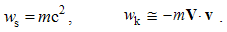 | (17.1) |
They express the potential energies of EM objects in the similar fields. With respect to the referent point – at infinity, the signs of the usual laws are kept. The approximate law (1b) is the special case of the kinetic law (2), strictly valid in the transverse direction only. In the longitudinal direction it understands the two equal speeds. On the other hand, the integration of the – more general – Lorentz’ kinetic force (12.12) gives mutual kinetic energy in the following more general form: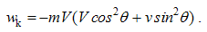 | (17.2) |
In the case of the equal speeds (V = v), it reduces to (1b). Unlike the static energy – in the symmetric form, the kinetic one depends on the polar angle, as the combined quasi-non- vortical field. Using the more operative expression (1b), we will keep in view its approximate sense.As the central forces per unit objects represent EM fields, respective energies per the same objects give the potentials. The laws (1) are thus resolved into the two potentials and respective energies of the objects in them: | (17.3) |
 | (17.4) |
The equations (3) express the field distributions, and (4) – respective energetic actions; the static quantities are at left, and kinetic – at right. Though seems formally more correct that the sign would belong to the potential, this convention appears more adequate in the continuation.If the general kinetic energy (2) were here used, with the square carrier speed in the longitudinal direction, the same potential would be obtained; only the kinetic energy in this direction would be distinct. With respect to these formal complications, the standard EM theory avoids the algebraic introduction of the potentials, but postulates a few gauge conditions as their inverse differential definitions from the fields. We will derive them from these ones.The alternative central laws are obtained by integration of usual, and so the fields are spatial derivatives of potentials. Really, some derivatives of the two potentials give the two respective (electric and magnetic) fields: | (17.5) |
The gradient is radial derivative of the static, ad curl – transverse derivative of kinetic potentials. These conditions express the fields as the differential characteristics of the potentials. The condition (5b) directly substituted into the dynamic Maxwell’s equation, relates the kinetic potential with the dynamic electric field: | (17.6) |
In the field form of force action law, the condition (6a) points to the reactive character of the dynamic electric field. The formal sum (6b) as the full electric field, affects all the present electric charges. On the other hand, the longitudinal derivative of (3b) gives its divergence: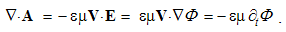 | (17.7) |
The electric field (5a) gives the convective derivative of the static potential (7). As the two odd functions – in the longitudinal direction, these both terms annul in the particle sequence of the line currents, i.e. ∇·A = 0.This chain of the equalities expresses the electric aspect of the kinetic potential. With respect to its transverse aspect (5b), it is called magnetic potential. The external continuity equation, relating the two EM potentials, is known as the intuitive condition of L. Lorentz. It points to the substantial interpretation of these two potentials.The comparison of their central distributions (3) gives the convective (8a), and equality of the two energies (4) – the relative relation (8b) of the two potentials: 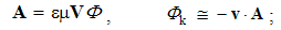 | (17.8) |
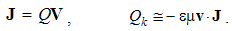 | (17.9) |
The central potentials substituted into (8), with volume derivatives of the discrete quantities, just gives (9) relating respective carriers. Apart from the dimensional harmony of the inversely related quantities, the two constants – as the medium elasticity and density – just explain the substantial interpretation of the two EM potentials.In the mechanical analogy of (1a), static potential, as the pressure disturbance, multiplied by medium elasticity and regular density, determines the density disturbance (εμΦ ). Its motion is equivalent to the linear momentum density (A), with respective kinetic (magnetic) energy.The above two pairs are analogous with respective field relations. The left pair defines the kinetic, by motion of the static quantities, and right – the equivalent reactions of the two kinetic quantities – on the moving objects. Though the transverse motion also causes some kinetic effects, it is not expressed by the two potentials, but by the fields – as their derivatives. This may be related with the defective energy (4b), used in the procedure of derivation.
17.3. Mutual Comparison
Let us compare the two alternative (8), with respective usual equations, convective and relative: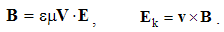 | (17.10) |
Apart from the uniform translation of non-vortical static field, (10a) also understands the radial contraction of the vortical dynamic field. The analogous former equation (8a) is restricted to the static potential and respective field. The usual equation (10b) understands the two directions of the object motion, perpendicular to the magnetic field, but (8b) is restricted to the longitudinal direction.In the domain of their common validity, the differential analysis of the alternative, just would give respective usual equations. Rally, div applied to (8a) thus emphasizes the longitudinal aspect of the vector potential: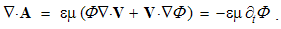 | (17.11) |
With the rigid potential around a moving charge, the former middle term annuls. The latter term represents the convective derivative of the potential (7).On the other hand, curl applied to (8a) emphasizes the transverse (magnetic) aspect of the vector A: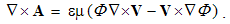 | (17.12) |
At the homogeneous speed, the former term annuls. With respect to (5a), the equation (10a) is obtained.Grad of (8b), with the annulment of all spatial derivatives of the homogeneous object speed, gives: | (17.13) |
In the form of Lorentz’ kinetic force, this is the sum of the longitudinal and transverse gradients. With the mutual (object-carrier) speed, v' = v – V, the former term may be generalized to the transverse direction. The potential vortex in the letter term represents magnetic field.
17.4. Moving Particle
Axial motion of the kinetic potential, together with its carrier, according to (6a) finally gives: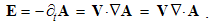 | (17.14) |
The potential is moving at speed V – in its own direction, with the same effect as that of the transverse contraction of its own vortex (B). Its longitudinal gradient, as convective derivative, accords to the divergence. The substitution of (7) into (14) gives the dynamic electric field: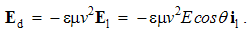 | (17.15) |
This axial field directed towards the carrier, is the former term of Lorentz’ force: f = q(E + v × B). As such, it deforms the static field into the ellipsoidal form. Scaled by the factor g = 1 – εμv2, the longitudinal field component tends to zero towards v = c. With respect to the invariant transverse field components, its full flux and electric charge tend to 2/3 of its regular values. Unlike the quark theory, the charge is not divided, but effectively gradually diminished.On the other hand, moving through its own magnetic field, a charge suffers respective transverse pressure, in the value of the latter Lorentz force term. The full kinetic force compresses the particle, thus increasing its mass. In spite of ellipsoidal field deformation, the even pressure is conserved. These two fields are also somehow related with the photon associated to the moving charge particle.With respect to vortical form of the total electric current, its convection part (qV) must be closed in the space by the same displacement currant: ∂tD = – V·∇D. The temporal is reduced to respective convective derivative. The family of its lines represents the associated photon, being the more convincing concept in relation to impossible wave packet. In the case of the gradual or rapid stoppage, it would be released from the particle. In the same form, it continues its own free propagation – at the speed c.The static potential in (3a) may be compared with some disturbance of the standard pressure in the elastic medium, alike cyclones and anti-cyclones in the atmosphere. Tending to the regular state, two equipolar particles mutually repel, and opposite ones attract each other. The typical medium features, elasticity (ε) and density (μ), identify the kinetic potential (8a) as the linear momentum density. The equation (6a) is nothing else but force action law. Bernoulli’s effect, as the transverse pressure loss in the flow (8a) is manifest as the magnetic field (5b), or the flow curl.
17.5. Summary
By resolution of the alternative laws, static and kinetic potentials are introduced. The latter of them results from the more operative, special case of the kinetic energy, keeping in view its general expression. In spite of the incomplete basis, the kinetic potential is correct. The two potentials are related differentially with the three EM fields. In absence of the clear insights, these relations were so far postulated as the gauge conditions. Their derivation here emphasizes both aspects of the vector potential, longitudinal – electric, and transverse – magnetic. They finally identify two EM fields as the formal features of the potentials.In parallel with algebraic relation of the two EM fields, respective potentials are similarly related. The derivations start from the central potentials and respective energies of the objects. The carriers are already identified as the formal features of the two fields. Unlike the cross-products relating the two fields, the scalar relations between potentials point to mechanical analogies: static as the pressure disturbance, and kinetic – as linear momentum density. This analogy is already implicitly used in electric circuits.Though the alternative set is narrower than usual, they are equivalent in the common domain of validity. Spatial derivatives of the latter set follow into the former one. The reduction of excessive terms understands the rigid, stably oriented potentials. In spite of their perpendicular motion, magnetic field and kinetic potential give the same results. The two terms of Lorentz force are related with the photon associated to a moving particle. In the form of a toroidal vortex, this model is superior to the wave packet and points to similar models of elementary particles.
18. Basic Sets
The field tensors determine 4D space as the ambient of EM processes. All the quantities are expressed in respective forms: potentials – as the vectors, fields – as bi-vectors and carriers – as tri-vectors. The static potential accords to the temporal, and kinetic – to three spatial axes; electric field to longitudinal, and magnetic – to transverse planes; electricity to xyz, and current to remaining 3D spaces. The quantities are related in two directions: of the same ranks algebraically, and between various ranks – differentially.
18.1. Introduction
Physical quantities express some motion of the physical substances (mass, energy & electricity), in respective spaces. Each of n1 subspace ranks in nD space enables respective motion: points – the rest, axes – translation, planes rotation, etc. For convincing presentation of the complex phenomena, their simpler analogy may be used. However, in spite of the successful application of the same differential operations of fluid mechanics – in EM theory, the analogy between their quantities is incomplete or multifold.In the classical mechanics, restricted to 3D space, mass and energy are the substances, their motion and forces are described by vectors, rotation & momentums by bi-vectors. The six subspaces of 3D space are thus used. A physical process is framed by respective space, as the ambient of its development. 3D space is thus sufficient for the mechanical motion. Due to inability of the motion and perception along additional axes, 5D space is restricted in experience – to its 3D projection, as the cosmos expanding along temporal axis. This universal expansion disables any other signals in this direction. The time is thus manifest by the sequence of temporal instants. The motion of a subject along fifth axis would mean respective transformation of his senses at least. Instead, the manifestations of inaccessible structural layers are transformed, by technical translation of the invisible – into visible signals.
18.2. Algebraic Equations
The algebraic equations relate EM quantities of the same ranks. Though needed for the full insight into the physical essences, they were unelaborated in the standard EM theory. Each algebraic pair relates (in both courses) respective two dissimilar quantities, electric and magnetic: | (18.1) |
 | (18.2) |
 | (18.3) |
 | (18.4) |
The left column represents the convective, and right – relative equations. The first pair relates the carriers, the two next – EM fields, and last – respective potentials. The double number of the field relations justifies their wide former elaboration and application. Let us further consider the two remaining pairs, the first and last.The first pair relates EM carriers, as the starting concepts, and last – EM potentials, as the essential quantities. The left pair expresses the motion of the static quantities, and right – their apparent kinetic reproduction. In fact, the right pair expresses transverse kinetic forces, in the terms of the static quantities. Unlike the simple current definition (1a), that of the potential (4a) is extended. It represents analogous linear momentum density, caused by the motion of some pressure disturbance in the medium. The two constants play the roles of elasticity and density of the medium. The static quantities may be treated as two bipolar substances. These relations are further explicated in the differential forms. Namely, div applied to (1a) & (4a) directly gives the two respective continuity equations: 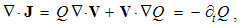 | (18.5) |
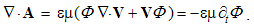 | (18.6) |
The divergence is resolved into dilatation and convection of the two scalar fields. At homogeneous speed, the former terms annul, and remaining – convective, give the temporal derivatives – at right. Divergences of the flows are reduced to the variable substantial densities. These variations are opposite to the moving field gradients.
18.3. Differential Equations
Unlike algebraic relations of the same rank quantities, the two successive ranks of – potentials, fields & carriers – are related differentially, by the following two triads: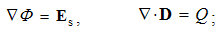 | (18.7) |
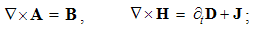 | (18.8) |
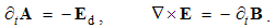 | (18.9) |
The left column relates the potentials with fields, and right – fields with carriers, including displacement currents. With respect to the non-vortical static and vortical dynamic fields, their sum (Es + Ed) may be understood.The first pair expresses static, second – kinetic, and third – dynamic interactions. They accord with respective three central laws, as the forces dependent on the position, motion and acceleration of punctual charges. In the absence of free magnetic poles and respective non-vortical field, the fourth (magneto-static) Maxwell’s equation is trivial, also without its pandanus amongst the left conditions.The inductive development of EM theory started from the assumed carriers and their associated fields, with the formal treatment of the two potentials. However, just the potentials represent the most real EM quantities, preceding the fields and, especially, carriers. The left column, defining the fields by potentials, supplements Maxwell’s equations – at right, defining the carriers by fields. The carriers are only the differential features of the fields, and the fields themselves – such features of the two potentials.Apart from the indirect relation of the two potentials and respective carriers – via EM fields, these two ranks of EM quantities can be related directly. Differential elimination of the fields from above sets relates these two ranks, as the 4D vector and tri-vector. The static (scalar) and kinetic (vector) quantities are separated by the equation (6): 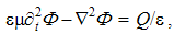 | (18.10a) |
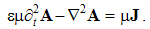 | (18.10b) |
The left terms of these equations, temporal and spatial, concern the static and dynamic electric fields, respectively. Namely, during this derivation, both of them are understood in all the three Maxwell’s equations. Mere substitution of (1,4-a) confirms the equivalence of these two equations. At non-conducting media, without free electric carriers, they reduce into respective wave equations.
18.4. Field Tensors
Relating the initial concepts, Maxwell’s set is usually applied. In the aim of its tensor generalization, it is here conveniently a little accommodated: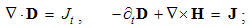 | (18.11) |
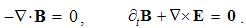 | (18.12) |
The pair (11) relates the fields with 4D current, where the charge moving along t-axis forms the fourth component. In the absence of the free magnetic carriers, the pair (12) is homogeneous. The two displacement currents are treated as the temporal field derivatives. Their opposite signs demand the negative sign of the trivial equation.Each curl-equation turns into three componential, thus giving the two sets of – by four equations each: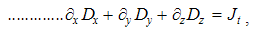 | (18.13a) |
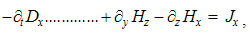 | (18.13b) |
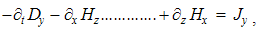 | (18.13c) |
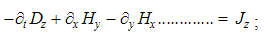 | (18.13d) |
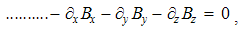 | (18.14a) |
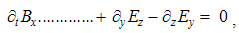 | (18.14b) |
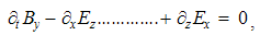 | (18.14c) |
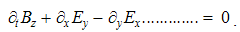 | (18.14d) |
The general indexes in the particular terms give the two Einstein’s equations, in the tensor form: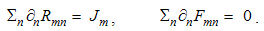 | (18.15) |
Index m denotes the ordinal number of the equation, with the summation per the index n ≠ m. The term senses are determined by the following field tensors: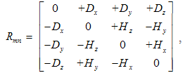 | (18.16) |
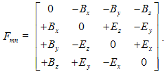 | (18.17) |
In the two ways, they identify 4D space as the ambient of EM processes. The distinct field locations point to the two levels of the observation. The former arrangement accords to the apparent electric carriers, with electric field in the longitudinal and magnetic – in transverse planes of 4D space. The opposite arrangement in the latter tensor accords to transparent magnetic carriers. The difference in their two relevancies speaks in favor of former tensor. On the other hand, the opposite signs of the temporal terms disable the assumed dual relation of these two tensors.With respect to the same numbers, there is the question of possible relation of the tensor and convective pairs. The four Maxwell’s equations, included into the tensor pair, are obtained by separate generalization of respective central field distributions. Unlike the differential pair – with the same wanted field, obtained from one convective, their synthesis into one tensor equation is crosswise. Therefore, the direct relation of the two pairs is impossible. However, the rational – contained in (2) and force fields – in (3) point to some parallelism between the two pairs.
18.5. Summary
This brief overview of the complete EM theory, points to the very solid scientific system. However, the multilateral parallelism of the basic physical quantities and their formal relations is not sufficient for elimination of any of them. Though mutually related in the algebraic and differential forms, all the quantities have their roles in the elaboration and exposition of EM theory. There follows their systematic correlation in the frames of 4D space, consisting of the three spatial and fourth temporal axes.All the quantities, in the vector and scalar forms, may be classified into 31 components – of the potentials and their carriers, mediated by 33 field components. These numbers accord to respective sub-spaces in 4D space: by four axes and 3D subspaces, with the six (2D) planes. Electric current and respective kinetic potential thus belong to 3D space, and their static components – to the temporal axis. In accord with the more relevant tensor (16), electric field belongs to the three longitudinal (xt, yt, zt), and magnetic – to the same number of transverse (xy, yz, zx) planes. All the quantities and respective subspaces are thus coupled.
19. Boundary Questions
There arise some boundary questions from the empirical features and mathematical relations of EM quantities. The reduction of static to kinetic EM forces expresses their unity, and comparison of static and dynamic electric fields points to the same manner of the force action. On the other hand, the explanation of EM potentials by the processes in the medium enables complete interpretation of EM quantities. On this basis, the structural models are proposed.
19.1. Introduction
The development of physics tends, and is finally reduced to the hunt for a basic structural particle, or for a set of them: from (indivisible) atoms, via elementary particles, up to the assumed quarks, of the senseless name. However, in the aim of their explanation & study, some structure of the vacuum medium, as the substratum of physical fields and substance of material particles, must been kept in view. With enough energy, a particle-antiparticle pair can be torn from vacuum, and also apparently annihilated or returned into it, releasing the energy invested into its formation.Inertial phenomena are here convincingly reduced to EM processes. On the other hand, EM fields and potentials can be explained by mechanics of the – compressible and inert – bound electricity. Electric charges or particles are their formal features only. The electric bipolarity reminds mutual interactions of the cyclones and anti-cyclones, formed in the atmosphere. In the medium structure, the forces are finally reduced to its thermodynamics. Some causal relations of the three classical disciplines may be established. The quantum mechanics is thus reduced to the empirical discipline, in the boundary region between two structural levels, with their analogous laws. The processes in the finer structure are observed by the instruments working on the cruder laws. Instead of the thermodynamics of the finer structure and its continual fields, this discipline operates by the cruder particles, their electrodynamics and mechanics. With respect to the incomplete former EM theory, quantum phenomena could not be explained, but were treated as the formal concepts or super-natural miracles.
19.2. Structural Models
In the aim of the deeper insight into 4D relations of the material structures constituted of the known particles, let us compare the interactions of two electric charges, described by the two central laws, static and kinetic: | (19.1) |
These laws express the two forces: only static – at rest, and the difference of static and kinetic ones – in the motion. The latter law is strictly valid in the transverse, but at the common motion – also in the longitudinal direction.The square of speed c in the former, instead of negative product of two collinear speeds – in latter laws, is the only distinction between them. Their unification can be obtained by means of two opposite speeds: V = – v. The static law appears as a special case of kinetic one, at equal opposite speeds. There is the question of the kinetic interpretation of the static force and respective electric field.The lapse of time points to the motion of all matter along the fourth axis. This axis may be set radially in the hipper- spherical cosmic model. Thus directed motion is projected as the expansion of 3D space. The speed c from (1a) points to the wave propagation. If the forth axis were closed into itself, as the three spatial axes, the cosmos would pulsate between some its maximal value and a singularity, without variation of the speed or direction of the wave propagation. Instead of the factor influencing the cosmic process itself, gravitation may be explained by its consequence, as the attraction of the parallel material flows.With respect to the flows in rt-planes, as the essence of electric field, the simplest model of a charge particle may be a hipper-toroidal vortex coaxial to t-axis. If the internal flow runs into the t-direction, the opposite external flow is closed into it, thus forming the vortex. In accord with CPT symmetry (circulation-polarity-time), all is opposite for the other polarity. The assumed redirection of the temporal axis would exchange the polarities of all particles. The uniform expansion secures the particle stability, as well as universal lapse of time, in accord with Galilean view.
19.3. Vacuum Medium
Elasticity and reactivity of the medium, with the regular mass density in its structure, are sufficient for the dynamic explanation of EM processes. The elasticity enables energy accumulation in some spatial locations. In the form of its reactivity, the medium tends to conserve its homogeneous density. Say that the overpressure accords to the positive, and under-pressure – to negative disturbances. The inertia and non-resistance of the medium maintain the motion of the images already formed in the vacuum medium. The two following equations thus start from the existent – static potential and its replacement through space: | (19.2) |
Static potential, followed by medium polarization, equals to zero in the undisturbed medium. If the disturbances are sufficiently small – in relation to the regular pressure, the variations are linear, with some equality of the two opposite potentials. The quantitative inequality of the two charges is conditioned by the opposite courses. Tending to the neutral medium, equipolar charges mutually repel, and opposite ones attract each other. The static force is expressed by the concept of electric field, as the gradient (2a). The medium is substratum of EM fields and potentials. With respect to the permanent particles and their fields, the features of reactivity and non-resistance are added to its elasticity and density. In the final instance, all these features are mutually causally related. Unlike the mechanical inertia already reduced to EM processes, these processes cannot be fully explained by the fluid mechanics, but electrodynamics of the medium is temporarily kept. Of course, the neutrality is finally reduced to the medium homogeneity.According to (2b), a moving disturbance represents some flow, as the kinetic potential. Its course also depends on the moving polarity. A moving negative particle, as the under- pressure, represents the opposite flow in the medium. In any case, each flow causes the transverse pressure loss. In EM theory this is expressed by the concept of magnetic field, affecting the other similar flows in the domain. The parallel flows mutually attract, opposite ones repel each other, but two crosswise tend to the same courses.Variation of speed or direction of the motion is followed by opposite reaction of the medium. This effect is expressed by EM induction, as the force action law: | (19.3) |
Mechanical inertia is already reduced to EM induction. With respect to the non-resistance of the medium, once obtained flows are further maintained.As the attraction of two parallel flows, respective force is expressed by the equivalent static potential (3b). The kinetic potential (A), as the moving disturbance, is here followed by another one, as the object of its action.
19.4. Temporal Domain
With respect to the medium, EM processes are reduced to its disturbances and their motion. A moving disturbance represents the linear momentum density. Its generalization to 4D space consists of the two components, temporal and spatial: A4 = At to + Ar ro . The former of them belongs to longitudinal planes (tr). Its motion along temporal axis, in the cosmic process, produces the static potential. The latter component represents the known kinetic potential, being contained and manifest in 3D space (xyz).The static electric field expresses the non-homogeneity of respective potential, and dynamic – the temporal variation of kinetic potential. The latter of them may be understood as the temporal gradient directed into the future: | (19.4a) |
 | (19.4b) |
Dimensional distinctions of the two axes are neglected, with co = 1. Added to the cosmic expansion, the temporal flow varies the transverse pressure – in 3D space, manifest as the static potential. With their formal similarity, the two electric fields mutually add: E = Es Ed. In 4D space they form the common vortices in rt-planes: | (19.5) |
Unlike the magnetic field axial to the vortex in 3D space, this is the polar vector, contained in the vortex plane, just determined by its cross-section with 3D space.
19.5. Summary
The model of a basic charged particle has all the features already expected. In fact, there is not any hard particle body, distinct from its fields and/or potentials, as the flows in the medium. The imagined membrane dividing the internal and external flows represents 3D particle surface, thus centrally symmetric and very elastic. Its radius is determined by the balance of the internal and external pressures on the surface. The former is ascribed to the centrifugal force of the vortex, manifest as the electric field. The external reaction of the polarized medium prevents the expansion.Though introduced arbitrarily, the two electric polarities are incorporated into the particle models. The internal flux of a positive particle is directed along temporal axis, and continued by the opposite external flux, and vice versa – at the negative particle. Added to the cosmic expansion, they cause opposite pressure disturbances, inside and outside, also opposite at the other polarity. The pressure difference on the surface thus results in the smaller radius and greater mass of a proton than that of electron. Exceptional stabilities of these two particles just speak in favor of their simplest elementary natures. They are the two sufficient elements for formation of the neutral structures of the atoms and their nuclei. Unlike a hydrogen atom, with the proton located in the center of the electron, neutron is the opposite combination of these two particles, of course, with the electron somehow compressed. The atomic nuclei thus represent the concentric alternation of the two particles, in the determined sequential orders.With respect to the displacement toroidal vortex around a moving charge, after liberation it represents the free photon. Unlike the hipper-vortices of the particles, photon is formed in 3D space, with axial motion in the frames of this space. The toroidal current is followed by the circular vortex of the magnetic field. Without static electric field, a photon does not manifest the charge and mass. The vortex reduced to one plane represents the polarized photon. The left and right photons do not distinguish in the experience, but their concentric combination forms a neutrino.At linear acceleration of a charge towards the speed c, its longitudinal electric field gradually decreases, and circular magnetic increases. By its form and structure, it is manifest as the associated photon. The boundary speed, with the zero particle radius, prevents its final transmutation into a photon. However, this event is possible with some help and direct participation of respective antiparticle.Unlike a massive particle, with its quantized charge and determined mass, a photon obeys the continual variation of its radius and frequency, related with energy: w = hν = ħω. Moreover, material motion along temporal axis represents the cosmos itself, as the moving medium of propagation of the photons. This relation points to the two distinct layers of the medium, as the substrata of the matter and light. The distinct subspaces of 4D space belong to respective layers of the medium structure, as their substrata.In this way, the particle-wave dualism of modern physics is explained and thus overcome. In the interactions with the instruments, the vortices are manifest as the particles or waves, but with their own natures ever kept.
20. Scientific Contributions
Instead of the two fields, EM phenomena are reduced to the three kinematical states – static, kinetic and dynamic – dependent on position, motion & acceleration of electricity. Three pairs of differential equations relate the three ranks of quantities: the potentials, fields and their carriers, presented in 4D by vectors, bi-vectors and tri-vectors. EM quantities of equal ranks are related algebraically. By the presented inductive elaboration, starting with the fields and potentials associated to their carriers, the inverse deductive exposition is enabled, in the opposite causal order.Taking the particles as the field sources or carriers, EM theory hesitated between the successive force transfer and direct distant action. Though the former view was adopted, all the equations implicitly understand the latter of them. Reducing the particles to mere centers of their fields, both views are here overcome. Algebraic equations describe the direct field actions, in each point of the space – separately, irrespective of the carriers. At least as the constituent parts of the particles, the fields are present in the whole domain, interacting directly and continually.Reducing EM theory to Maxwell’s equations, a reference frame for the field motion is avoided. On the other hand, restricting to the inertial frames, the dynamic processes are also tried to avoid. Apart from the problematic definition of these frames, the reference of the speed in the mass function was tacitly ignored. Instead of the subjective orientation, in relation to the observer or his instruments, the objective approach concerns the medium of EM processes. By Mach’ principle, this medium is ascribed to the gravitation of a dominant, or – of more relevant bodies.With respect to convincing EM indications, the temporal axis is clearly interpreted. Mounted radially to the hipper- spherical cosmos, it points to its continual expansion, in the cosmic wave form. As such, it just determines the universal and uniform lapse of time. The global spatial curvature is thus clearly explained. On the other hand, by the medium stratification, in the form of zooming in and out – of its structure, the fifth axis is here introduced. It is demonstrated by Poynting’s theorem, as the 5D continuity equation, with the spatial, temporal and substantial terms.A few antinomies, arisen from the unresolved physical problems, are overcome. Instead of dual nature of photons and massive particles, their vortical models are proposed, as the syntheses of the two former alternatives. The manifest features of these two entities depend of the angle of their observation, without any mystics. Moreover, instead of the phase and group speeds of light propagation, the two new terms, wave and effective speeds, just announce respective interpretation. The accumulating medium layer slows down the propagation through the transferring layer.A vacuum medium, already denied in SRT, is reaffirmed. The new particle model, as the vortex of the displacement current, points to the solid resting medium. The particles and their compounds are nothing else but dielectric images in this medium. The speed of the cosmic expansion is just determined by the medium features, and light propagation – by similar features of this moving medium. With respect to the empirical facts, it consists of the gravitational potentials of all celestial bodies. A repeated copy of the primary in the secondary images may be expected.During 200 years of development and application of EM theory, all the measurable facts are already tested. At least some of thus obtained results are merely here explained. Though accords to Maxwell’s static equation, Faraday’s cup is here widely interpreted, as the absolute neutrality of the space. The opposite disturbances of various structural layers mutually annul at each point. This explanation is the basis of the fifth dimension, enabling similar generalization of the action-reaction law, to the absolute energetic homogeneity, also equivalent with the energy conservation.Two additional Faraday’s results are also interpreted. The signal arisen in a rotating magnet or disc in its front, do not obey the usual concepts of EM induction. These effects are here reduced to the magnetic interaction of the two parallel currents: magnetization one – on the magnet cover, and the convection current of free electricity in the rotating material. These phenomena are strictly mathematically treated. Other explanatory attempts are also denied, as is the extension of relativity principle beyond its frames, here restricted to the transverse direction of the line conductors. Faraday’s twisted polarization in the axial magnetic field is reduced to Fizeau’s effect. The circular vector potential plays the role of the rotating medium, dragging the wave propagation in its own direction. The two negative results, of Trouton-Noble & Michelson-Morley, origin from a same principal error. Using the victorious heliocentric orientation, they lost from view the dominant gravitation of Earth in the observed location. Of course, the Sun’s influence is decisive concerning the planets, as the objects, being subjected to its dominant gravitation in the wider space.The general kinetic law is finally obtained. Not only that the expected torque on a moving dipole does not obey the action-reaction symmetry, but the relativity principle must be taken into account, in the frames of its validity. Apart from the manifest object speed, that of the carrier field must be subtracted from it. There was an implicit antinomy: the resting field would fall behind its own carrier, but moving with it would cancel the kinetic interaction between the two poles. Certain transverse field motion, here proposed and explained, just satisfies all the conditions.Lorentz’ mass function, formulated from the empirical diagrams, is here strictly obtained from the force balance on the particle surface. This function and Einstein’s equation are confirmed and interpreted on EM bases, without any mystification, used in SRT. The mass, being equivalent to the electrical energy around charge particles, is increased by the particle compression, caused by the new force balance on the surface. At checking of its radius, the elastic electron surface was not taken into account, thus opening the door for the later relativistic speculations.Basic algebraic equations are systematically introduced, fully elaborated and applied. The convective pair describes production of one, by motion of other EM field, and relative – their reactions on dissimilar moving objects. Relating the variation and motion, a complementarity of the convective and differential equations is established. On the algebraic bases, the complete field transformations are formulated. Founded on the incomplete transformations, SRT is finally disproved, excepting the two above dynamic relations. The deformations of space and time are excluded.The methodical sequence of transparent thematic lessons enables the gradual acceptance of the new ideas and results, starting from the usual views and knowledge. Not only that such a convincing exposition is the main condition for the successful presentation and easy acceptance of the theory, but it was the dominant method during the 30 years of this investigation. The well founded formal and interpretative arguments speak in favor of the obtained results. Starting from Maxwell’s theory, the contributions were compared with the empirical facts already well-known.
References
| [1] | Essential Overview of EM Theory, Springer-Verlag, Selected Topics in Nonlinear Dynamics and Theoretical Electrical Engineering, Volume 459, Chapter 13, 2013. |
| [2] | Inductive Elaboration of EM Theory, SAP, Int. Journal of Electromagnetics and Applications, 3(3), 2013, |
| [3] | Deductive Exposition Foundation of EM Theory, SAP, Int. Journal of Electromagnetics and Applications, 3(2), 2013, |
| [4] | Thematic Consideration of EM Theory, SAP, Int. Journal of Theoretical and Mathematical Physics, 3(3), 2013, |
| [5] | Systematic Foundation of EM Theory, SAP, Int. Journal of Electromagnetics and Applications, 4(1), 2014, |
| [6] | Basic Laws of EM Theory, SDI, Physical Science International Journal, 4(10), December 2014, |
| [7] | Axiomatic Presentation of EM Theory, SAP, Int. Journal of Electromagnetics and Applications, 5(1), 2015, |
| [8] | Boundary Questions of EM Theory, SAP, Int. Journal of Theoretical and Mathematical Physics, 4(3), 2014, |
| [9] | Medium of Natural Phenomena, SAP, International Journal of Theoretical and Mathematical Physics, 4(4), 2014. |
| [10] | Relativity and/or Symmetry, SAP, International Journal of Theoretical and Mathematical Physics, 4(5), 2014. |
| [11] | Final Essence of Material Existence, SAP, International Journal of Theoretical and Mathematical Physics, 5(1), 2015. |
| [12] | Space, Time and Motion, SAP, International Journal of Theoretical and Mathematical Physics, 5(1), 2015. |
 Abstract
 Reference
 Full-Text PDF
 Full-text HTML