H. R. E. H. Bouchekara 1, 2, H. Allag 2, 3, M. Boucherma 2
1Department of Electrical Engineering, College of Engineering and Islamic Architecture, Umm Al-Qura University, P. Box: 5555, Makkah, 21955 Saudi Arabia
2Electrical Laboratory of Constantine “LEC”, Department of Electrical Engineering, Mentouri University Constantine, 25000, Constantine, Algeria
3LAMEL Laboratory Jijel University BP 98 Ouled Aissa, 18000 Jijel, Algeria
Correspondence to: H. R. E. H. Bouchekara , Department of Electrical Engineering, College of Engineering and Islamic Architecture, Umm Al-Qura University, P. Box: 5555, Makkah, 21955 Saudi Arabia.
| Email: |  |
Copyright © 2012 Scientific & Academic Publishing. All Rights Reserved.
Abstract
The study of Electromagnetics is required in most electrical engineering graduate and undergraduate curricula. Traditional methods for teaching Electromagnetics are abstract, theoretical and filled with large number of mathematical equations. Thus, they are not anymore appropriate. The solution is to provide to both professors and students an interactive software with a simplified graphical interface to best teach and learn fundamentals of Electromagnetism. Interactive resources have demonstrated that they were attractive and encouraged the students to be active and autonomous. The aim of this work is to present such interactive software. This software introduces the students to fundamentals of Electromagnetics and provides them with better ways to understand complicated concepts. It uses the calculation functions of Matlab, combined with the powerful graphical user interfaces of Java.
Keywords:
Electromagnetics, Matlab/Java, Electromagnetic Education
Cite this paper: H. R. E. H. Bouchekara , H. Allag , M. Boucherma , Software for the Support of Learning and Teaching in Electromagnetics, International Journal of Electromagnetics and Applications, Vol. 1 No. 1, 2011, pp. 1-6. doi: 10.5923/j.ijea.20110101.01.
1. Introduction
The electromagnetic theory based on Maxwell’s equations in integral and differential forms is considered to be fundamentally important in the undergraduate education of electrical and electronic engineers. The typical pattern for an undergraduate course is that of progression from static field concept to the dynamics laws, followed by applications. Most undergraduate books, whether inductive[1] or axiomatic[1], first develop the theory of completely static electric and magnetic fields and ending up with dynamic electromagnetic field theory[1]. The electrical engineering department at Umm Al Qura University is developing a course sequence that will allow students to get essential basics of Electromagnetics. However, the electromagnetic Engineering education, in particular requires the assimilation of large amount of math by the students. The very nature of the study of electromagnetics requires development of a strong theoretical foundation. For students, this is often challenging[2]. Thus, many students prefer not to study Electromagnetics if given a choice. They question its relevance since interesting, ‘real world’ problems are difficult to cover in an introductory course[3]. They also complain that Electromagnetics is too theoretical and abstract, that is simply another mathematics field course with a jumble of dry, uninteresting and confusing equations[3]. The most notable changes in how we teach EM are the visualization and animations of fields through software and instrumentation which have strongly impacted the way students learn Electromagnetics and its applications, today[4]. A number of researchers have suggested the use of computers to assist in teaching Electromagnetics[3][5]. Electromagnetic softwares can be considered as a possible supplement to traditional electromagnetic courses[6]. The ability to add visualizations, rapid solutions and practical skills into the curriculum is appealing[6]. Many packages exist which prove to be extremely powerful and useful in this approach, but they are so powerful and general that they often need a university course by themselves to be mastered and even their basic utilization can be too long to learn within a standard course devoted to Electromagnetics[7].A solution can be made by costuming specific programs, with a simplified possibly graphical interface, which can be presented very quickly leaving the greatest possible time to learn Electromagnetics. The purpose of this work is to present an interactive Electromagnetics software called EMSoft (Electro Magnetics Software). It is a combination of Matlab and Java. Matlab is an efficient software which put the powerful calculation function, visual and program designing together in an easy used development environment. Java is a cross-platform program development language which is created by Sun. It is the most advanced program language which also has the richest characteristic and has the most powerful function. In EMSoft, Matlab is used for all calculation functions, visualization and scripting, and java is used to generate useful interactive User Interfaces.The remainder of the paper is organized as follow: section 2 introduces the concept of the EMSoft and its environment. In this section the main interface and the main features of this software are presented. Section 3 illustrates how to use EMSoft by considering 4 detailed examples. These examples are respectively chosen from the vector analysis filed, from the electrostatics field, from the magnetostatics field and the last example is to illustrate advanced applications. Finally, the overall paper conclusion is drawn in Section 4.
2. The EMSoft Computer Software Environment
The core of EMSoft has been developed under MATLAB for Windows applications. As the m-files written for MATLAB are not compiled into binary form, students are also able to see the inner structure of the program and have the chance to see how an Electromagnetics software is implemented on a computer. This can inspire some students to make their own program or even develop their own software. JAVA is one of the most popular programming languages at present. It has huge libraries to develop useful and powerful interfaces. For the development of interfaces JAVA has been used. So, JAVA is combined with Matlab to give more ability and flexibility to EMSoft. The structure of EMSoft is given in Figure 1.When EMSoft starts, the first window that appears is the Model Navigator as shown in Figure 2 This is a starting point where the user can use models from the existing library (Model library) or create new models (User Library). Two other tabs allow the use of this software for other applications (Advanced and Assignments Tabs). | Figure 1. EMSoft environment. |
2.1. Model Library
There are four main Library Models which are namely: Vector Analysis: Vector analysis is a mathematical tool with which EM concepts are most conveniently expressed and best comprehended. Actually, students must first learn vector analysis rules and techniques before they can confidently apply it. Since most students taking this course have little exposure to vector analysis, this library model will considerably improve students understanding of vector analysis. In this model library, students can test and/or extend their knowledge on the basic concepts of vector algebra in the main coordinate systems (Cartesian, cylindrical and spherical). This model library will also help students to be familiar with operations on vectors; starting from basic principle like addition, subtraction, and multiplication (dot product, cross product, triple scalar and vector products) and going through integration and differentiation including important principles as gradient, divergence, rotational and Laplacian.Electrostatics: The important properties of time independent static electric fields are exposed in this second model library. It includes forces between stationary charges, electric field (due to point charges, line charges, surface charges and volume charges), electrostatic potential, electric dipoles, flux lines, equipotential surfaces, and the electric energy. So, this library model exposes clearly the two basic laws of Electrostatics; Coulomb and Gauss laws.Magnetostatics: In this model library the students can review the magnetic effects that will be encountered if the charge is in motion with a constant velocity that can be described as being a current. So, several procedures to calculate the magnetic field can be used. Forces between two current elements can also be calculated in this model. This model makes an emphasis on Biot-Savart and Ampere laws. Time Varying Electromagnetic fields: This model is an extension of the static electric and magnetic fields to time varying fields. Students can explore mostly two new concepts: the electric field produced by a changing magnetic field and the magnetic field produced by a changing electric filed (Faradays and Maxwell works). Each one of these major four models is composed of several sub-Models. For example, the main model Electrostatics is composed of sub-models as Coulomb’s force, Ampere’s circuit law, and so forth. The selection of an appropriate sub-Model opens a new interface and allows to put (or/and change) the different parameters, then run the simulation (see section 3). The results can be exposed as numerical values (magnitudes of forces for example) or as a 3 dimension rotatable drawing (for example, position of points or vectors, forces, flux lines, etc.).
2.2. User Models
For example, if the students have a project in which they will combine different library models, or work with particular or advanced models, for easy access, they can create their own user model libraries. If a model image is saved along with a description they appear in the Model Navigator when the specified user model is selected. If there is HTML based documentation for the model, the Documentation button allows viewing it.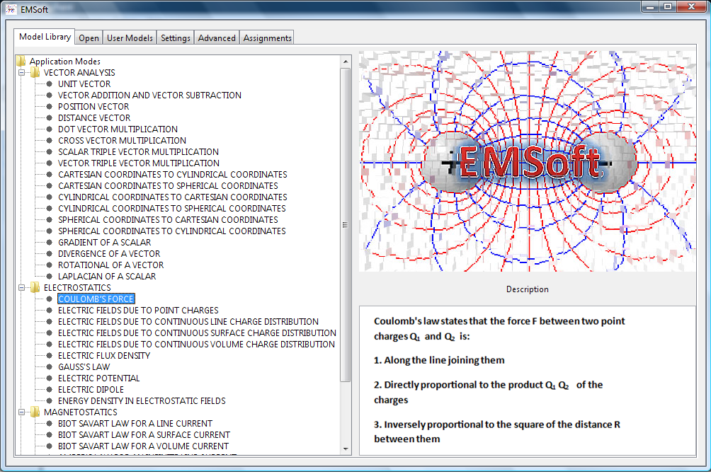 | Figure 2. The main interface of EMSoft |
2.3. Advanced
This tab can be used in students research projects, where solving partial differential equations (PDE) is needed. Students can choose between finite differences and finite elements methods to solve their problems. In future development of the software the magnetic moment method can also be integrated.
2.4. Assignments
Added recently to EMSoft, this tab is a very interesting part of the program. It is very useful for both students and professors. In the case of students, they can generate homework assignments using the assignments library. They can simulate test exams (by generating test exams where the problems are selected or randomly chosen from a specified list of problems) or they can check their answers in actual exams by submitting the exam to the program corrector. However, not all exams can be submitted to the corrector.For professors, they can generate some problems to put into the exams. Web-based learning tools are indispensable in modern teaching, especially when the ability to reveal extra information on demand is an excellent tool for stimulating and engaging students. This is why this part of the software should be extended o the web.
2.5. Settings
In this tab the students can choose the language (English or French). In this version of EMSoft English and French are the languages that exist but this can be extended to Arabic, Spanish, Italian, German, etc.). This tab allows changing the look of the EMSoft by changing the general Look and Feel, the background and the fonts (style and color). In this tab the students can also change the unit systems and put the one that fit their needs.
2.6. Postprocessing and Exporting data
EMSoft provides tools for plotting and postprocessing any model quantity or parameter:Surface and contour plots (for example: electric and magnetic field densities, electric and magnetic fluxes, etc.).Arrow plots (for example: electric and magnetic forces, EM fields, etc.).Cross-section plots and numerical interpolation.Animations (for example: the electric field of a moving charge, the variation of magnetic forces on a rotating current element, etc.)Export solution data to text files and script workspace. Postprocessing allows the students to analyze results and make the link between the concepts taught during the lecture and their exploitations (more details are given in section 3).EMSoft supplies a number of tools for zooming, orbiting, and panning to adjust the view of a model for postprocessing, and general visualization.
2.7. Help
A full documentation of EMSoft is available with the software. In this help several examples can serve as a start point for students to be familiar with the program.
3. Examples and Applications
Example 1: Illustration of the gradient, the divergence and the rotational using EMSoft scripting and Interfaces.Assume that there exists a surface that can be modeled with the equation: | (1) |
Let’s use EMSoft to illustrate the profile, to calculate and plot this field. The gradientCartesian2D command is used to compute the gradient of z in the 2 D Cartesian coordinate system. It gives: | (2) |
The contours with the same value are connected together and the resulting field is indicated in Figure 3 (a). The length of the vectors and their orientation clearly indicate the distribution of the field in space as shown in Figure 3 (a). The divergence of the 2D vector field:  | (3) |
where r has as components x and y so  and α=const is present in Figure 3 (b). In addition to the divergence scalar contours Figure 3 (b) shows the plot of the 2D vector filed by EMSoft.Using EMSoft, the rotational of the 2D vector field:
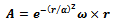 | (4) |
where r has as components x and y so  and
and  is illustrated in Figure 3 (c) by contours. While the plot of the 2D vector filed is illustrated by arrows.
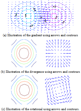 | Figure 3. Illustration of the gradient, the divergence and the rotational using EMSoft |
We can use also the EMSoft interfaces to calculate the gradient of a scalar. Let’s find the gradient of the following scalar field: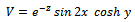 | (5) |
Using the interface shown Figure 4 (a) we can enter the expression of the scalar V. The result is calculated and displayed in Figure 4 (b) and given in (6).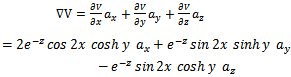 | (6) |
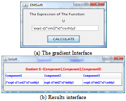 | Figure 4. Calculation of the gradient of a scalar using EMSoft |
Finding the divergence of a given vector can also be performed using EMSoft. If we take for instance the vector Q (in cylindrical coordinates) given by: | (7) |
Using the interface shown in Figure 5 (a) we can enter the 3 components of the vector Q. A check is automatically done to identify in which coordinates system the vector is given (in this case; cylindrical coordinates). Then, the calculations are performed with respect to this coordinate system. The result is calculated and displayed in Figure 5 (b) and given in (8).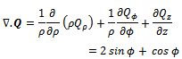 | (8) |
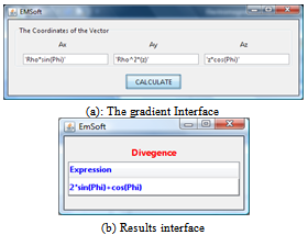 | Figure 5. Calculation of the Divergence of a vector using EMSoft |
Example 2: Illustration of Coulomb’s law using EMSoft interfacesA full documentation of EMSoft is available with the software. In this help several examples can serve as a start point for students to be familiar with the program.Coulomb’s law states that if there are N point charges located, respectively, at points with position vectors
 , the resultant force F on a charge Q located at point r is the vector sum of the resultant force F exerted on Q by each of the charges
 . Hence:
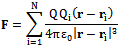 | (9) |
To illustrate this fundamental EM law, let’s calculate the force on a 1nC charge located at  caused by four identical 3nC charges located at
  ,
,  ,
,  and
and  as show in Figure 6(a).The Figure 6 (b) shows the interface to edit such problem by giving the amount of charges and where they are located. The results are illustrated in Figure 6 (c). This result interface gives the force exerted by each of the four charges
  ,
,  ,
,  and
and  on
on  (where the force has to be computed). Each force is represented in the table by its three components and its magnitude.
  . The last column of the table corresponds to the resulting force which is the sum of all forces.
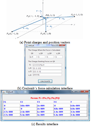 | Figure 6. Illustration of Coulomb’s law using EMSoft |
 | (10) |
Finding the vector  in this equation is not always easy. A simple approach is to determine
  as:
as: | (11) |
where a1 is a unit vector along the line current, ρ is the perpendicular distance between the line current and the point where the magnetic field is computed and ao is the unit vector along the perpendicular line from the line current to the field point.Our experience in teaching Elcetromagnetics shows that students have many difficulties to identify ρ and ao. To compute ρ and ao they have to imagine the whole configuration in 3D which is not evident for all students. EMSoft can help students to visualize the whole configuration in 3D with different views (top, bottom, right left and perspective views).To show that let us take a basic example, a current filament carrying 15 A in the az direction lies along the entire z axis. The question is to find H in cartesian coordinates at  .From Figure 7, it is clear that the four shown views help to compute ρ and ao. One can see the projections of the point P on the line carrying the current. Thus;
 | (12) |
And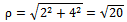 | (13) |
The current line is along the z axis, thus,  . So:
. So: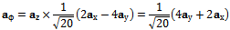 | (14) |
The magnetic field created at P is equal to: | (15) |
Example 4: Illustration of Advanced applications.For advanced applications the design of the synchrounes electrical machine is selected as an example. The Finite element method (FEM) is applied to the synchrounous machine with saillent and non saillent configurations.Figure 8 shows the main steps (geometry drawing, meshing, resolution and postprocessing) for the design and modeling of such machine by using the FEM.Electromagnetic design problems usually involve a large number of varying parameters. A designer (or a student) can use different kinds of models in order to achieve optimum design. Some models, e.g., finite-element model, can be very precise: however, it requires large computational costs (i.e., CPU time)[8]. Therefore, the designer should use a screening process to reduce the number of parameters in order to reduce the required computational time. The benefits of this technique are tremendous[9]. 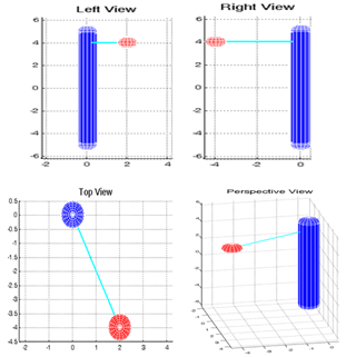 | Figure 7. EMSoft views window |
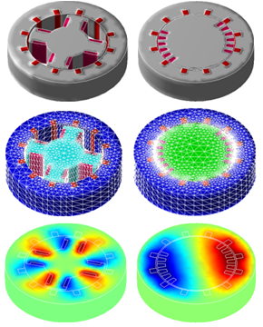 | Figure 8. EMSoft Advanced applications |
For an efficient use of the DOE methodology, it has been implemented in the form of interactive tool called Design of experiments Tool. It receives the output from the simulation model and automatically processes this output using the DOE technique. Thus, this tool can be used interactively via EMSoft either to give advice to the user conducting the simulation study, or else to directly control simulations.
4. Conclusions
The complexity of problems from the field of EM makes their understanding and study difficult for students. Computer programs like EMSoft allow students to better understand the main EM topics. EMSoft is simple, flexible and powerful software for helping students to overcome the challenge imposed by EM courses.While using Matlab in EMSoft gives a powerful modeling environment by using all Toolboxes already there in, JAVA and its huge API Libraries are used for the development of EMSoft interfaces.
References
| [1] | Lumori, M.L.D.; Kim, E.M., "Engaging Students in Applied Electromagnetics at the University of San Diego," IEEE Transactions on Education, vol.53, no.3, pp.419-429, Aug. 2010 |
| [2] | Venkataraman, J.; , "Project based electromagnetics education," Applied Electromagnetics Conference (AEMC), 2009 , vol., no., pp.1-4, 14-16 Dec. 2009 |
| [3] | S.L. Broschat, J.B. Schneider, F.D. Hastings, Steeds, M.W., ‘In-teractive software for undergraduate Electromagnetics’, IEEE Transactions on Education, Vol. 36, Issue 1, pp.123 – 126, February 1993 |
| [4] | Emson, C.R.I.; Edwards, J.D.; , "Using commercial design software as an aid for teaching electromagnetics," Computation in Electro-magnetics, 2008. CEM 2008. 2008 IET 7th International Conference on , vol., no., pp.68-69, 7-10 April 2008 |
| [5] | Yuan Bin, Nakata, T., Wang Hengli, Liang Changhong,‘An agent-oriented system for self-programming electromagnetic field analysis software’ IEEE Transactions on Magnetics, Vol. 35, Issue 3, Part 1, pp, 1678 – 1681, May 1999 |
| [6] | Mills, A.K.; Chappell, W.J.; , "On the use of commercial FEM electromagnetic software in an undergraduate curriculum," Antennas and Propagation Society International Symposium, 2004. IEEE , vol.3, no., pp. 3365- 3368 Vol.3, 20-25 June 2004 |
| [7] | S. Selleri, ‘A Matlab application programmer interface for educational Electromagnetics’, Antennas and Propagation Society International Symposium, IEEE Vol.3, pp.450 - 453, June 2003 |
| [8] | H. Bouchekara, G. Dahman, M. Nahas ‘‘Smart Electromagnetic Simulations: Guide Lines For Design of Experiments Technique’’ Progress In Electromagnetics Research B, Vol. 31, 357-379, 2011 |
| [9] | H.R.E. Bouchekara, M.T. Simsim, Screening applied to the numerical modeling of electromagnetic devices, Ain Shams Engineering Journal, Volume 1, Issue 2, December 2010, Pages 131-137 |
 Abstract
 Reference
 Full-Text PDF
 Full-text HTML