1. Introduction

An early assumption of the theory of rocky shore communities was that there are no stabilizing responses by the ochre sea star (Pisaster ochraceus) on the population of its main prey, the California mussel (Mytilus californianus). Instead, it was believed that physical factors, mainly desiccation stress, kept sea stars from foraging for mussels in a spatial refuge high on the shore [1]. It was thought that the vertical foraging ranges of sea stars were fixed by the tidal regime: the upper shore level being the refuge, or safe zone, for mussels, whereas the lower shore level was considered to be the zone accessible to sea stars. Thus, the assumption was that there is no biotic regulatory interplay based on reciprocal responses between sea stars and mussels, as observed in other predator-prey interactions. Subsequent experiments showed that some mussels were able to escape predation by sea stars, not because of a spatial refuge, but because these mussels grew large enough to resist the predatory activities of sea stars.

In 1959, C.S. Holling published a study on the numerical and functional responses exhibited by predators based on prey availability [2]. A numerical response is characterized by an increase in predator density whenever prey density increases. A functional response occurs when a predator kills more prey in response to an increase in prey availability. Holling demonstrated that desert rodents show an increase in density and predation rate in response to an increase in the density of their prey Symphyta (sawfly), thereby keeping the prey from completely populating the local environment. More recent studies suggest that Pisaster may have similar behavioral responses to changes in mussel abundance. A juvenile mussel transplantation experiment [3] demonstrated that Pisaster has the ability to aggregate in areas of high mussel recruitment and disperse in areas of low mussel recruitment, which is suggestive of a numerical regulatory response by sea stars. This aggregative response by sea stars, in addition to an increase in predation rate with an increase in mussel density, a functional response, helps to keep the mussel population in check. Another observation that exemplified the stabilizing regulation by sea stars is that variation in mussel recruitment has the potential to cause huge fluctuations in the lower intertidal zone if no predators were present, but such fluctuations are seldom observed under natural conditions.

A predatory response that has been proposed, known as the developmental response, is defined as a predator’s ability to consume more prey in proportion to the size of the predator [4]. A predator that is capable of a developmental response exhibits plasticity of growth. That is, as the predator continues to feed, it will increase in size allowing it to increase its predation rate. A predator that is capable of a developmental response has the ability to change its feeding habits as it grows by eating larger prey, alternate prey, or by an increase in its predation rate. In the case of the sea star/mussel interaction, as a sea star grows, it will increase its predation rate on the mussel population. On the other hand, in the case of very low prey density or very small prey size, a predator that exhibits plasticity of growth will shrink to a small size. Theory predicts that predators that are capable of exhibiting numerical, functional and developmental responses will be able to stabilize a prey population more effectively than predators that only exhibit a subset of these predatory responses [5].

In 1970, Howard Feder conducted experiments to study the plasticity of sea star growth [6] and found that average sea star size in a particular location is related to the abundance and size of prey at that site. A relationship between the size of a sea star and the prey it eats exists because the energy provided by the environment depends on the size and density of prey. Feder demonstrated that a primary reaction of sea stars to starvation is a loss of body mass instead of death. As prey density increases, more energy is available in the environment to sustain sea star growth.

To simulate the plasticity of growth of sea stars, an ODE-based model was derived to account for predator competition for prey due to a large predator density or due to low prey density. The model is used to simulate experiments similar to those performed by Landenberger [7] and Menge [8], where dead mussels were continuously replaced with adult mussels of the same size in order to keep the average mussel size and mussel density constant. The model also simulates experiments where average mussel size is kept constant, mussel density is allowed to vary over time, and there is a constant mussel recruitment rate. The derivation of the mathematical model is based on energy flow mechanisms and is presented in the Materials and Methods section. Stability and bifurcation analyses are presented in the Results section, followed by suggestions for improving the model in the Discussion section.

2. Materials and Methods

The individual growth rate of a sea star is based on a balance of the energy flow mechanisms that are known to affect sea star growth. The following assumptions were made to derive the model:

1.An open system where the prey recruitment is independent of mussel density and sea stars do not leave the region (mussel patch) regardless of prey density.

2.Mussel growth rate and mortality due to natural causes are negligible.

3.Sea star size and mussel size are assumed to be the average values of each population.

4.New mussel recruits are assumed to be adult mussels of constant size.

5.Environmental disturbances affecting predator mortality or foraging activity were not considered.

6.It is assumed that competition for prey is negligible when predator density is low, but competition becomes intense at high predator densities.

2.1. Energy Flow Mechanisms in a Sea Star

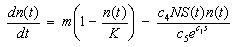
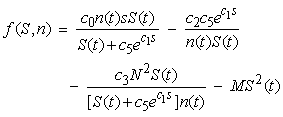
Field experiments [9] have demonstrated that given a group of keystone predators, a large majority of them will feed when there is prey abundance, but only a small portion will feed during periods of prey scarcity. Rapport and Turner [10] suggested that Pisaster ochraceus is an energy maximizer. That is, this sea star does not feed at its physiological maximum rate but, instead, this species consumes prey at a rate that maximizes its net energy gain. Therefore, energy flow plays a significant role in determining the growth of a sea star. While sea stars obtain energy from the environment by consumption of mussels, they also lose energy through a variety of mechanisms. For example, sea stars use energy while foraging and handling prey and by sustaining metabolic processes. A sea star will grow (increase in diameter) if its net energy gain is sufficient to promote growth. A sea star will shrink in size if the energy loss is greater than its energy gain. Based on previous experimental observations [6-8], [11], energy flow mechanisms provide a sound explanation of the observed growth of sea stars in response to variations in prey biomass (abundance and average size). The net change in sea star size over time due to energy gain or loss can be represented by the following equation

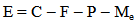(1)

where the terms of the equation are defined as follows

C: change in sea star size per unit time due to energy gained through consumption of mussels,

F: change in sea star size per unit time due to energy loss through foraging and handling of mussels,

P: change in sea star size per unit time via energy loss due to competition with other sea stars for food resources, and

M_e: change in sea star size per unit time via energy loss due to sustained metabolic processes.

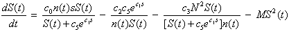
2.2. Modeling the Growth Rate of Sea Stars

Energy flow mechanisms affect the net energy gain (or loss) that drives sea star size growth (or shrinkage). The model uses an equation similar to the one described in [10] that incorporates all of these energy mechanisms. Equation 2 models changes in average sea star size over time:

(2)

In the discussion that follows, n(t) and N are the densities of mussels (number of mussels per m²) and sea stars (number of sea stars per m²), respectively, while s and S(t) represent the size (in cm) of mussels and sea stars, respectively.

2.2.1. Energy Gain Due to Mussel Consumption

We let c₀ be a coefficient that relates average energy gained by a sea star through consumption of mussels having biomass n(t)s, to individual sea star growth. Mussel resistance to predation increases exponentially with an increase in mussel size s and is represented by the term [9, 10], where c₁ is a coefficient relating mussel resistance to predation to mussel size. The dimensionless factor represents the predation efficacy of a sea star. The constant c₅ is a weighting factor used to adjust the units for dimensional consistency. Since larger sea stars consume more mussels as a consequence of their developmental response, this means that the predation efficacy increases with an increase in sea star size S(t) if mussel size s is kept constant. On the other hand, since an increase in mussel size leads to a higher predation resistance, the predation efficacy of the sea star decreases with an increase in s. The fact that a larger mussel biomass n(t)s provides more calories for sea stars is represented in equation 3, which describes the energy gain of a sea star through mussel consumption

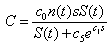(3)

A higher mussel biomass creates an environment that can support sea stars of larger size and density. In the model, mussel density was included in the expression for energy cost as a variable that affects foraging (search time) cost, as explained in the next section.

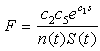
2.2.2. Energy Cost of Foraging and Handling of Prey

Sea stars spend energy searching for prey and this foraging cost is reduced when mussels are abundant. The smaller the mussel density, the greater the distance sea stars have to travel to search for food items, thus increasing the foraging cost. The expression represents the inverse relationship between foraging cost and mussel density. The coefficient c₂ relates mussel density to energy spent through foraging. In addition, the expression

(4)

is a dimensionless factor that represents the predation resistance of a mussel of size s relative to sea star size S(t), and this ratio determines the energy cost of handling prey experienced by a sea star. It has been shown that in sea star-mussel interactions prey-handling time increases with mussel size [11, 12]. Sea stars may experience a higher energy loss when trying to consume relatively large mussels, since their prey-handling time will increase. Consequently, a larger sea star will spend less energy foraging and handling prey than a smaller sea star. This leads to the following equation representing the total foraging and prey handling cost F incurred by a sea star:

(5)

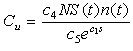
2.2.3. Energy Cost Due to Competition for Prey

Whenever sea stars share a common resource, they will compete directly for food via intraspecific or interspecific agonistic behavior [13, 14], or will compete indirectly by depriving their competitors of food items [8]. A large group of sea stars equipped with a good predation efficacy may reduce or deplete food items in a particular region, which leads to an increased search time for other sea stars due to the fact that they now have to forage farther out to find suitable prey. Therefore, the energy cost due to competition between predators increases as the predation efficacy increases.

Mussel density n(t) influences the energy cost by sea stars due to competition for prey, since mussel density determines food availability in the environment and affects the foraging time of sea stars. A quadratic term N² was used to model the assumption that competition for prey is negligible when predator density is low, but becomes very intense at high predator densities. The expression for the total energy cost due to competition for prey is given by

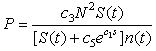(6)

where c₃ is a coefficient that relates the total energy cost due to competition for resources to the three main factors: predator density, predation efficacy, and prey density.

2.2.4. Energy Cost Due to Metabolic Processes

If one assumes that the energy cost due to metabolism M_e is proportional to the surface area of a sea star, and represent its surface area by S²(t), then a larger sea star will spend more calories per unit time to sustain metabolic processes. This assumption is represented by the equation

(7)

where M is a coefficient relating metabolic energy cost to the surface area of a sea star.

2.3. Changes in Mussel Density

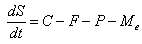
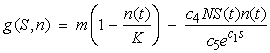
Sea stars experience a growth or reduction in size in response to changes in prey biomass n(t)s. Under natural conditions, mussel biomass varies in the intertidal zone according to gradients that include mussel recruitment rate, tidal height, and wave stress. In the model, mussel density n(t) was allowed to vary over time, and changes in mussel density over time were incorporated in the model to account for the variability of mussel biomass in naturally-occurring mussel beds. A density-dependent logistic growth model for mussel population growth was considered as described in [15]. The mussel population growth rate R tends toward zero when mussel density n(t) approaches the maximum carrying capacity K = 400 mussels / m² of the environment. The mussel population growth rate is high when mussel density is low. The rate of change of the mussel population depends on a balance between mussel growth rate R and the mussel consumption rate C_u by sea stars. The rate of change of the mussel population is represented by the equation

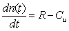(8)

where

(9)

and

(10)

Here, m represents the mussel recruitment rate, while the coefficient c₄ relates mussel consumption to predator biomass, mussel density, and mussel resistance to predation.

Based on the above analysis, the following two-dimensional ODE model was derived to describe the change in average sea star size and the change in the mussel population in a dynamic biological environment:

This system of ordinary differential equations was used to study the effect of sea star competition for prey on the developmental response of sea stars to changes in prey biomass.

3. Results

3.1. Graphical Stability Analysis

In Cases 1 – 3, prey density was kept constant at the environmental carrying capacity of 400 mussels / m². It was assumed that all the mussels have the same size and that a mussel that is killed by a sea star is immediately replaced with an adult mussel of the same size. By holding prey density constant, the effect that a change in predator density N has on the terminal size of sea stars was investigated. The parameter values used in the model simulations are listed in Table 1 and were estimated based on empirical evidence.

(11)

(12)

Table 1. Parameter Values

3.1.1. Case 1: N = 1 sea star / m²

By holding sea star density constant at N = 1 sea star / m², the model predicted an asymptotically stable equilibrium for average sea star diameter of 42.7 cm, and an unstable equilibrium of cm. This prediction is shown in the plot of growth rate dS/dt versus size S in Figure 1A, and in the plot of size S versus time t shown in Figure 1B. In terms of energy flow mechanisms, this environment does not lead to a net energy gain that is sufficient for sea stars to grow beyond 42.7 cm. Sea stars with an initial size larger than 42.7 cm will adapt to environmental conditions by shrinking. The model predicts that very small sea stars will have a hard time killing mussels and, consequently, it will take them much longer to grow and reach the stable equilibrium size of 42.7 cm. Although such a large sea star size is not common in nature, sea stars of a comparable size have been observed [16]. A large predicted terminal sea star size is plausible in this simulated environment, given that it consists of a high mussel density and competition between sea stars is negligible due to the low predator density. The sea stars don’t need to forage at all to find their prey due to the high mussel density. In this scenario, mussels 10 cm long are a significant source of energy and the prey handling cost incurred by the sea stars is not excessively high.

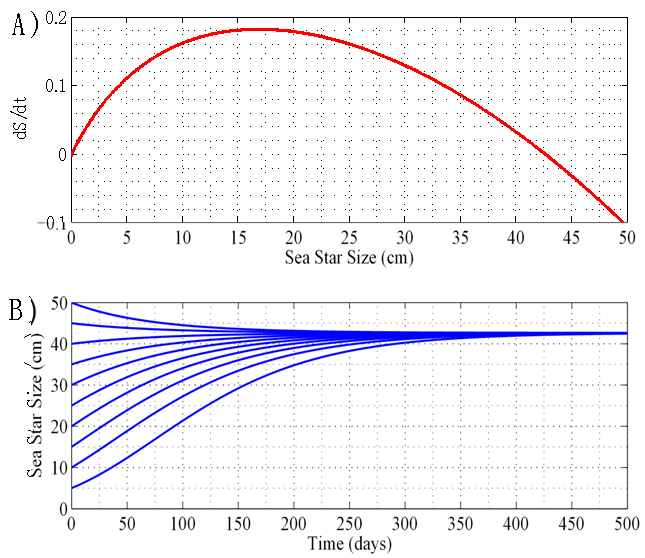Figure 1. A) Sea star growth rate dS/dt versus sea star size S for N = 1 sea star / m2. B) Corresponding plot of sea star size S versus time t. Sea stars of different initial sizes grow or shrink to the same terminal size of 42.7 cm in diameter

3.1.2. Case 2: N = 8 sea stars / m²

In this scenario, sea star density was increased to N = 8 sea stars / m². The model predicted a sea star diameter of S = 32 cm to be asymptotically stable and S = 0 cm to be unstable. This prediction is shown in the plot of growth rate dS/dt versus size S in Figure 2A, and in the plot of size S versus time t shown in Figure 2B. These results indicate that an environment characterized by a constant large supply of mussels having a size of 10 cm, can support a relatively large sea star density of N = 8 sea stars / m². In this scenario, competition for prey increased considerably, leading to a smaller average sea star size due to the cost of intraspecific competition. The predicted terminal size of 32 cm, although smaller than the sea star size predicted in Case 1, was still relatively large. This result can be attributed to the fact that in Case 2 sea stars were surrounded by a dense bed of mussels and, thus, did not have to spend much time looking for prey.

Since the stable equilibrium value for average sea star size decreased with an increase in sea star density from N = 1 to N = 8, it is expected that the stable equilibrium value for S will approach the unstable one (cm) as the predator density N is increased, since no environment can support an infinite number of sea stars due to predator interference and competition for prey. There must exist a predator density N_b such that the predators and prey will be unable to coexist if i.e. sea starts will shrink to a size so small that they will no longer be able to prey effectively on mussels and would no longer be considered predators of mussels. An objective of the stability analysis was to identify the value N_b that produces the predicted bifurcation.

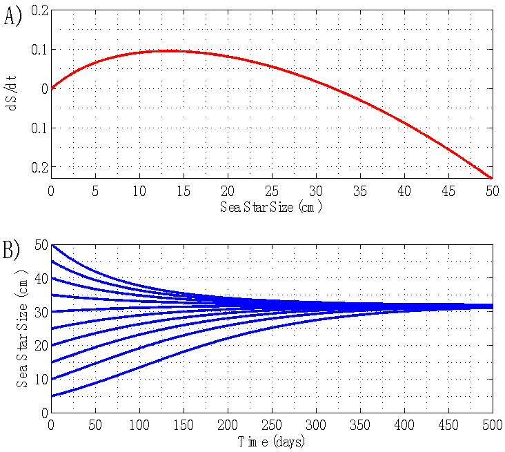Figure 2. A) Sea star growth rate dS/dt versus sea star size S for N = 8 sea stars / m2. B) Plot of sea star size S versus time t. Sea stars of different initial sizes grow or shrink to the same terminal size of 32 cm in diameter

3.1.3. Case 3: N = 12.62 sea stars / m²

When sea star density was increased to 12.62 sea stars / m², the system underwent a bifurcation characterized by a coalescence of the stable and unstable equilibrium points. The plot of growth rate dS/dt versus size S in Figure 3A shows that the curve fails to intersect the positive side of the x-axis. The consequence of this bifurcation is that if sea stars / m², sea stars of any size will decrease in diameter (Figure 3B) and their long-term size will approach zero (a globally stable equilibrium). The fact that sea star size tends toward zero does not necessarily mean that the sea stars will die. Experimental observations have shown that sea stars can survive without food for months [6]. The model predicts that sea stars survive by shrinking to reduce metabolic costs, while sacrificing their mussel predation efficacy. Tiny sea stars are no longer considered predators of mussels and, at this point, predator-prey coexistence disappears. Based on the predictions of the model, a predator density of 12.62 sea stars / m² is too large for the specified environmental conditions of this scenario to be a source of net energy gain for a sea star of any size. In nature, it is possible that when average sea star size is large and sea star density is high, agonistic behavior will occur between sea stars. These combative actions may lead sea stars to experience a high energy cost due to competition for prey. Eventually, these sea stars will shrink to a size so small that they will be unable to prey on the mussels and will shrink even further, thus explaining why cm became an asymptotically stable equilibrium point.

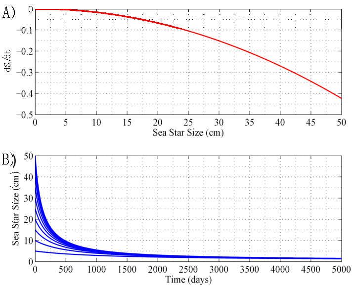Figure 3. A) Sea star growth rate dS/dt versus sea star size S for N = 12.62 sea stars / m2. B) Plot of sea star size S versus time t. Sea stars of all initial sizes shrink to a very small size due to the intense competition for prey caused by a high sea star density

Figure 4 depicts a bifurcation plot for the model as predicted by cases 1 – 3. The bifurcation plot shows that for N < 12.62 sea stars / m² the system has two equilibria: a stable equilibrium value for sea star size S (representing predator-prey coexistence) and an unstable equilibrium value . The two equilibria coalesce when N = 12.62 sea stars / m². For N > 12.62 sea stars / m² the only stable equilibrium is . This means that, given a very large sea star density, sea stars will shrink to a small size due to their energy being spent on agonistic behavior against each other, as well as intraspecific competition for mussels. Once sea stars shrink to a very small size, they will no longer be able to kill adult mussels and the sea stars will remain small.

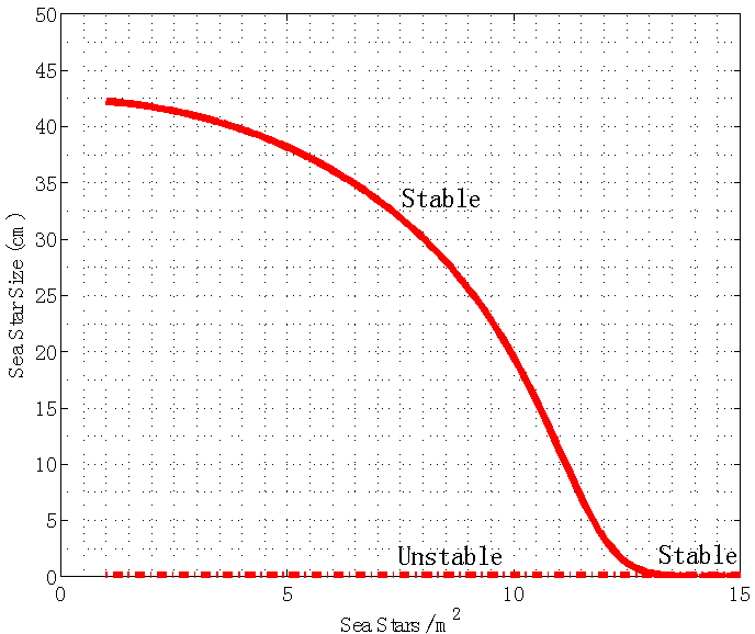Figure 4. Bifurcation plot of sea star size S versus sea star density N when mussel density n(t) is kept constant at 400 mussels/m2. All other parameters were held at the default values shown in Table 1. When predator density is increased to N = 12.62 sea stars / m2, a bifurcation occurs and the stable and unstable equilibria coalesce into a single globally stable equilibrium point

Other model parameters, including prey density and prey size, were varied to determine their effect on terminal predator size. The model predicted an average terminal sea star that is an increasing function of mussel density. On the other hand, the terminal sea star size increases to a maximum size of 42.7 cm in diameter as mussel size increases from 1 cm to 12 cm. A mussel size less than or greater than the optimal size of 12 cm leads to a smaller terminal sea star size. A decrease in sea star size is to be expected for very small mussels, since small mussels may not be a significant source of energy for a sea star to attain a large size. A decrease in sea star size is also to be expected for very large mussels, since the availability of only large mussels increases the prey handling cost incurred by a sea star significantly. These predictions are shown in Figure 5. The plasticity of sea star growth makes terminal size a function of mussel biomass n(t)s. It is known that mussel biomass varies under natural conditions due to gradients in tidal height and wave stress that affect average mussel size and density [17]. Sea stars are indeterminate growers and their individual growth seems to be limited by seasonal spawning [6] and by food supply [8], but not necessarily by a physiological absolute maximum size limit. Since sea stars are energy maximizers, they grow or shrink to a size that maximizes their energy intake in a particular environment.

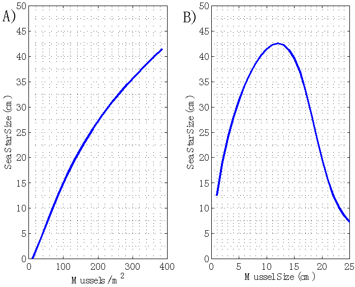Figure 5. A) Terminal sea star size S as a function of mussel density n. Sea star size is predicted to increase as mussel density increases, since an increase in mussel density decreases both predator competition for prey and the foraging cost. B) Terminal sea star size S as a function of average mussel size s. The model predicts an optimal mussel size that leads to the largest terminal sea star size

In Cases 4 – 6 discussed next, prey density was allowed to vary over time in order to investigate the predator characteristics and environmental conditions that lead to a stable predator-prey coexistence. The parameter values used in the model simulations are listed in Table 1.

3.1.4. Case 4: N = 1 sea star / m²

When sea star density was fixed at N = 1 sea star / m² and mussel density was allowed to vary, two equilibrium points were obtained, one stable and the other unstable. A phase portrait of mussel density n(t) versus sea star diameter S(t) is shown in Figure 6, where both n(t) and S(t) represent dynamical variables specifying the state of the predator-prey system at time t. Trajectories that flow towards the stable equilibrium (asymptotically stable node) show that, given the environment specified by the parameter values, sea stars and mussels can coexist, with sea stars predicted to have a terminal size of 28.8 cm in diameter, while the mussel population will reach an asymptotic density of 205.6 mussels / m². The unstable equilibrium (saddle) occurs when cm, which means that no sea stars capable of preying on mussels are present, allowing mussel density to approach the carrying capacity of 400 mussels / m². In Figure 6, the vertical trajectory going up along the vertical n-axis is a branch of the stable manifold of the saddle point (S*, n*) = (0 cm, 400 mussels / m²), and it confirms the fact that in the absence of a keystone predator such as the ochre sea star, mussels are able to colonize the entire substrate and are capable of excluding other species from the area.

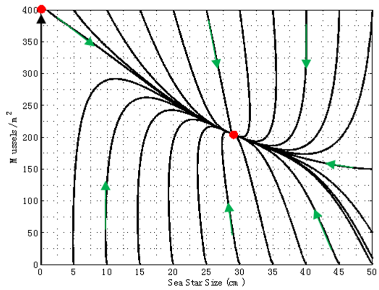Figure 6. Phase portrait of mussel density n(t) versus sea star size S(t) assuming a constant predator density of N = 1 sea star / m2. The equilibrium point (S1, n1) = (28.8 cm, 205.6 mussels / m2) is an asymptotically stable node, while (S2, n2) = (0 cm, 400 mussels / m2) is a saddle

3.1.5. Case 5: N = 5 sea stars / m²

In this scenario, predator density was increased to N = 5 sea stars / m². Figure 7 shows that sea stars and mussels can still coexist in spite of the increased sea star competition for mussels. The model predicts an average terminal sea star size of 8 cm and a smaller mussel density of 172.5 mussels / m², thus simulating the regulatory effect of sea stars on the mussel population. Large sea stars will shrink due to increased competition, and the faster depletion of prey due to the developmental response of large sea stars. The trajectories shown in the phase portrait illustrates the capability of sea stars of growing, or shrinking, to a size that will maximize their net energy gain while still allowing them to keep the mussel density in check. The unstable equilibrium (saddle) corresponds to an average sea star size of cm (no sea stars capable of preying on mussels are present), in which case mussel density will increase to the carrying capacity along the stable manifold of the saddle point.

Figure 7. Phase portrait of mussel density n(t) versus sea star size S(t) assuming a constant predator density of N = 5 sea stars / m2. The equilibrium point (S1, n1) = (8 cm, 172.5 mussels / m2) is an asymptotically stable node, while (S2, n2) = (0 cm, 400 mussels / m2) is a saddle

3.1.6. Case 6: N = 11.68 sea stars / m²

Increasing predator density to N = 11.68 sea stars / m² produced a bifurcation of the equilibrium points into a single globally stable equilibrium point (S*, n*) = (0 cm, 400 mussels / m²). The decrease in average sea star size to cm is due to intraspecific competition for prey. The trajectories of the phase portrait in Figure 8 show that as mussel density decreases, sea stars experience an increase in predation cost due to competition for prey. This energy cost outweighs any energy gains made by sea stars while foraging, and will result in a net reduction in average sea star size to a very small size cm. Consequently, there will be an increase in mussel density up to the mussel carrying capacity. A group of sea stars that is initially large is able to reduce mussel density to a greater extent than a group of small sea stars. In both cases sea star size approaches zero due in part to competition for prey when sea stars are large, and due to small sea stars being unable to prey on mussels that are 10 cm long.

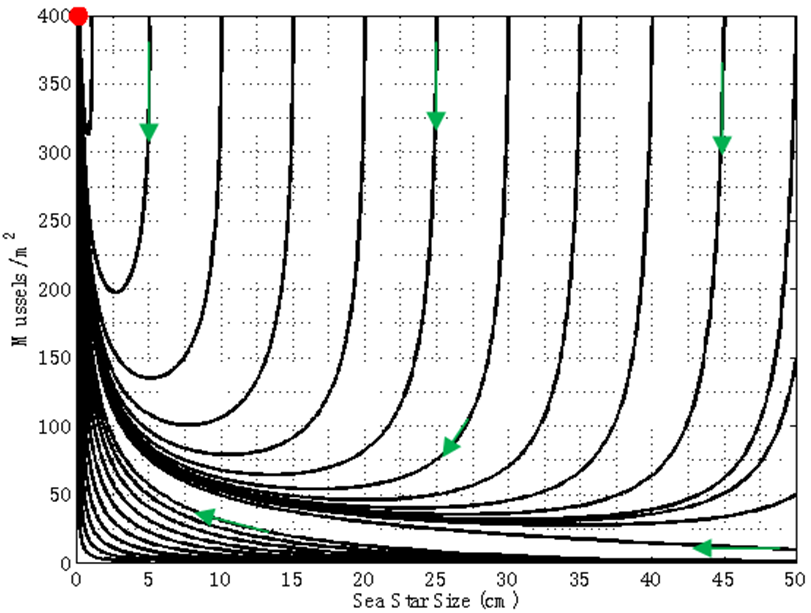Figure 8. Phase portrait of mussel density n(t) versus sea star size S(t) assuming a constant predator density of N = 11.68 sea stars / m2. The only equilibrium point (S, n) = (0 cm, 400 mussels / m2) is globally stable

Figure 9 depicts a bifurcation plot of sea star size S versus sea star density N as predicted by Cases 4 – 6. This bifurcation plot shows that for N < 11.68 the system has two equilibria, a positive asymptotically stable equilibrium value for S and an unstable equilibrium value cm. At N = 11.68 the two equilibria coalesce. For N > 11.68 the only stable equilibrium is cm, in which case sea stars of any size will shrink to reduce the direct competition for prey, and to decrease the metabolic cost incurred when a sea star has a large body size. In an actual intertidal setting, tiny sea stars may feed on alternate prey or stop foraging altogether and remain small.

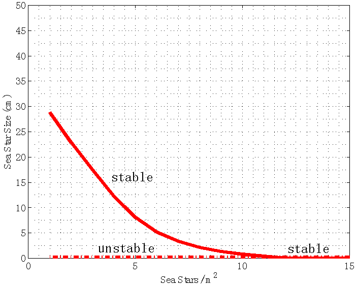Figure 9. Bifurcation plot of sea star size S versus sea star density N when mussel density n(t) varies over time. All other parameters were held at the default values shown in Table 1. The bifurcation occurs when sea star density is increased to N = 11.68 sea stars / m2, in which case coalescence of the stable and unstable equilibrium points occurs. Notice that when prey density n(t) is allowed to vary over time, the terminal sea star size decreases faster as sea star density increases compared to the bifurcation plot in Figure 4 when prey density was held constant at the carrying capacity of the environment

In Case 6, if the average mussel size is larger than 12 cm, an asymptotically stable equilibrium for sea star size that is not close to zero is predicted. In fact, when mussel size was set at s = 20 cm, the asymptotically stable equilibrium point was approximately (S*, n*) = (8 cm, 320 mussels / m²). This result shows that a large average mussel size can offset some of the cost due to competition for prey, allowing the coexistence of predator and prey.

The rate of mussel recruitment m also determines the asymptotically stable value for sea star size and mussel density. Depending on how large the mussel recruitment rate is, sea stars may or may not be able to keep mussels from dominating the intertidal zone, even when sea stars have a large initial size. Figure 10A shows that as recruitment of new adult mussels increases, sea stars will attain a larger terminal size. The model predicts that as sea star density N increases, the terminal sea star size will decrease due to an increased competition for prey. Although a high sea star density can hinder the developmental response by sea stars through competition for prey, a high sea star density can also help to stabilize a mussel population that exhibits a high recruitment rate. However, the long-term mussel density will first decrease and then increase if the density of sea stars continues to increase. For example, if predator density is very high (N = 9 sea stars / m²), this will lead to the same long-term mussel density predicted by the model when N = 1 sea star / m², as shown in Figure 10B.

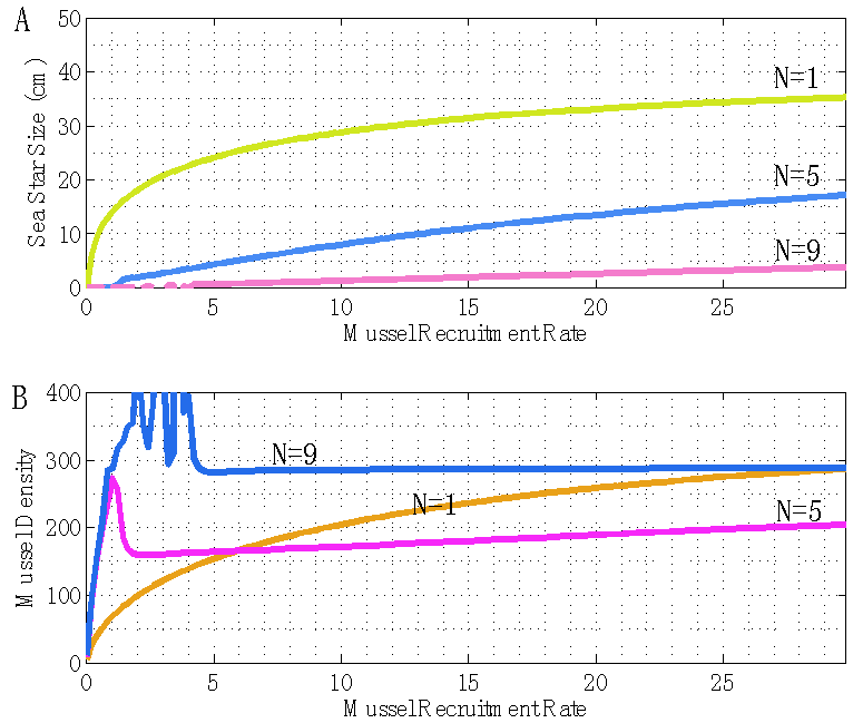Figure 10. Plot of terminal sea star size S and mussel density n(t) versus mussel recruitment rate m. A) As mussel recruitment increases, the terminal sea star size is predicted to increase. As sea star density increases, the terminal sea star size will decrease due to an increased competition for prey. B) As mussel recruitment increases, the long-term density of mussels is predicted to increase. As sea star density increases, the long-term density of mussels will initially decrease but then it will increase. This result illustrates the capability of sea stars of stabilizing a fast-growing population of mussels through a predatory developmental response if competition for prey is not too intense, and the negative effect that intense predator competition (N = 9 sea stars / m2) for prey has on the stabilization of the prey population by predators

3.2. Analytical Stability Analysis

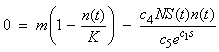
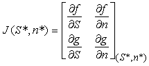
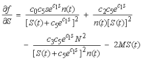
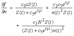
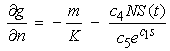
An analytical stability analysis was conducted to verify the results of Cases 4 – 6. The equilibrium points (S*, n*) were computed by setting and in equations (11) and (12) and solving the following system of nonlinear algebraic equations for S(t) and n(t) simultaneously:

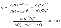(13)

(14)

Next, the nonlinear system of ODEs representing the model were linearized around each equilibrium point by computing the Jacobian matrix evaluated at each equilibrium point, along with its corresponding determinant, trace and eigenvalues (shown in Table 2). The Jacobian matrix was computed by first expressing the right side of equations (13) and (14) as functions of S(t) and n(t):

(15)

(16)

and constructing the Jacobian matrix J by computing the following partial derivatives

(17)

where

(18)

(19)

(20)

(21)

(22)

(23)

The following are the Jacobian matrices for Cases 4 – 6 evaluated at each equilibrium point when mussel density was allowed to vary.

Case 4: N = 1 sea star / m²

(S₁, n₁) = (28.8, 205.6)

(S₂, n₂) = (0.031, 399.6)

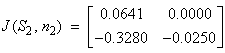Case 5: N = 5 sea stars / m²

(S₁, n₁) = (8.0, 172.9)

(S₂, n₂) = (0.033, 397.8)

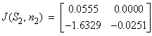Case 6: N = 11.68 sea stars / m²

(S, n ) = (0, 400)

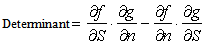
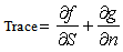
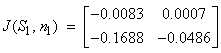
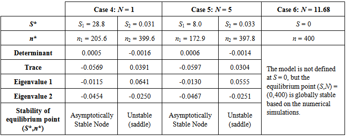
Table 2 shows that when sea star density equals 1 sea star / m² and mussel density is allowed to vary over time (Case 4), the equilibrium point (S₁, n₁) = (28.8 cm, 205.6 mussels/m²) in Figure 6 is an asymptotically stable node, since the determinant is positive and both eigenvalues are real negative numbers. This stable equilibrium point represents coexistence of predator and prey. The equilibrium point (S₂, n₂) = (0.031 cm, 399.6 mussels/m²) is a saddle because the determinant is negative. This means that in nature, mussel density will approach the environmental carrying capacity via the stable manifold (the n-axis) in the absence of predatory sea stars, or in the presence of sea stars that are too small to kill any mussels. A small perturbation about the point (0.031 cm, 399.6 mussels/m²) represented by the presence of predatory sea stars, will reduce the mussel density to the asymptotic value of 205.6 mussels / m². In Case 5, when sea star density was fixed at 5 sea stars / m² and mussel density is allowed to vary over time, the equilibrium point (S₁, n₁) = (8.0 cm, 172.9 mussels/m²) in Figure 7 is an asymptotically stable node because both eigenvalues are real, negative numbers. On the other hand, the equilibrium point (S₂, n₂) = (0.033 cm, 397.8 mussels/m²) is unstable.

Table 2. Stability Analysis of the Equilibrium Points

The bifurcation of the equilibria occurs in Case 6, when predator density N is set to 11.68 sea stars / m². In this scenario, the only equilibrium point is (0 cm, 400 mussels/m²), as shown in Figure 8. Although the model is not defined at S = 0 cm, it can be concluded that the equilibrium point (0 cm, 400 mussels/m²) is globally stable based on the numerical simulations of the graphical stability analysis. A high predator density leads to a fast depletion of resources (available mussels), coupled with an increasing competition between the predators. As a consequence, as and the average sea star size will become so small that these tiny sea stars will be unable to prey on mussels. This, in turn, leads to an asymptotic mussel density of 400 mussels / m². Based on the results of the graphical and analytical stability analyses, the model predictions correspond to what is expected to occur in nature.

4. Discussion

The analysis of the model presented in this article yielded information on conditions leading to predator-prey coexistence when the predator is capable of a developmental response to changes in prey density. It was also shown that the stabilizing effect of an increase in sea star density N is possible only for a particular N range. However, the stabilizing effect of sea stars on the mussel population can persist in spite of a very large density, if characteristics of the mussel population change (e.g an increase in average mussel size). The key factor that seems to determine coexistence is whether a keystone predator such as Pisaster ochraceus can obtain sufficient energy from the mussel biomass to achieve a terminal size that will allow it to kill prey efficiently. The availability of energy in the environment changes over time whenever mussel recruitment, mussel density or mussel size change. Since the present model assumed a constant mussel recruitment rate m and a constant mussel size s, it will be useful to reformulate the model by redefining these constant parameters as variables of the model. This modification to the model will lead to a more realistic prediction of the changes in mussel biomass n(t)s(t) and average sea star size S(t) over time.

Although three different responses by sea stars to changes in mussel biomass are possible (numerical, functional and developmental), the analysis of this model focused only on how predator competition for prey affects the developmental response and the resulting system dynamics. Introducing an equation that simulates the change over time of the predator population P(t) will make it possible to investigate the effect of a numerical response by predators on the stability of predator-prey dynamics. Keeping track of changes in mussel killing rates by sea stars will make it possible to study the effect of a functional response on the sea star - mussel interaction. The objective of future work will be to incorporate the three predatory responses to simulate their synergistic effect, as has been done in [5], to determine the conditions under which this synergism of predatory responses can overcome, or can contribute to, the destabilizing effect of predator competition for prey.

Mussel populations are affected by stochastic fluctuations in mussel recruitment [18] and environmental effects that lead to dislodgement of mussels from a patch [19, 20]. Cooperative aggregation and anti-predator defenses by mussels also play a role on the stability of mussel beds [21, 22]. The ODE model presented in this article did not consider these aspects of the mussel population. A stochastic model that considers spatial neighborhood effects could be formulated to incorporate key aspects of mussel population dynamics together with spatial predator foraging and competition for prey. The stochastic model can then be used to investigate the extent to which mussel intraspecific cooperativity can lead to stable predator-prey coexistence, and the extent to which stochastic recruitment can destabilize sea star-mussel interactions.

5. Conclusions

A deterministic model of sea star growth based on energy flow mechanisms predicted the asymptotic average sea star size as a function of sea star density, mussel recruitment rate and mussel size. These parameters determined the intensity of competition that predators experience and the energy (via prey biomass) available in the environment. The graphical and analytical stability analyses confirmed the existence of an asymptotically stable equilibrium for sea star size and mussel density in which both predator and prey can coexist, demonstrating the capability of a stabilizing response by sea stars. The predictions of this model were consistent with experimental evidence showing that predatory sea stars have the capability of a developmental response, characterized by an increase in feeding rate, as a result of an increase in size, which allows them to stabilize a mussel population. The model also predicted that intense competition for prey between sea stars can hinder their developmental response to the point of rendering them unable to control a mussel population. A bifurcation value for predator density was identified, below which the system exhibits multiple equilibria and predator-prey coexistence is possible, and above which the system exhibits a single equilibrium point that is globally stable. In the latter scenario, predator-prey coexistence disappears, with mussels populating the entire substrate and attaining a density equal to the environmental carrying capacity.

Conflict of Interests

The author declares that there is no conflict of interests regarding the publication of this article.