1. Introduction

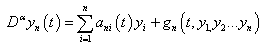
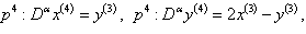
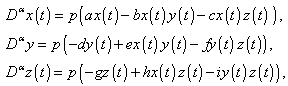
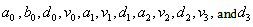
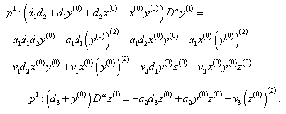
Ecosystem models play an important role to know the dynamics of the system. Such models are formed by combining known ecological relations with data gathered from field observations ([1]-[8]). These models are then used to make predictions about the dynamics of the real system. However, the study of deficiencies in the model leads to the generation of hypotheses about the possible ecological relations that are not yet known or well understood. Models enable researchers to simulate the conclusions of large-scale experiments that might be too expensive to perform on a real ecosystem. These also enable the simulation of ecological processes over very long period of time (may be some process may take centuries of time in reality), However this can be done in a matter of minutes in a computer model. Ecosystem models have applications in a wide variety of disciplines, in particular, to natural resource management. An important aspect any model evaluation is the validation, that is, the process of confirming that the model behaviour corresponds to reality. The results of the model can be validated by comparison with field data, but this technique limits the validation to a particular set of field conditions. We obtain a sequence of equations in which the solution at any stage is close to the solution at nearby stages. In the present paper we discuss the fractional Ecosystem model and solve it using Homotopy Perturbation Method.

We consider the following fractional ecosystem model given by fractional initial value problem of the type:

with initial conditions Here f and

g are arbitrary functions, denotes the fractional derivative in the sense of Caputo.

2. Basic Definitions

In this section, we give the related definitions and properties of the fractional calculus from [9].

Definition 2.1. A real function is said to be in the space if there exists a real number where , and it is said to be in the space if and only if

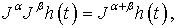
Definition 2.2 The Riemann–Liouville fractional integral operator of a function, is defined as

is the well-known Gamma function.

Some of the properties of the operator , which we need here, are as follows:

For

(1)

(2)

(3) .

Definition 2.3. [10] The fractional derivative of in the Caputo’s sense is defined as

for

The following are the two basic properties of the Caputo’s fractional derivative [10]:

(1) Let is well defined and

(2) Let

This leads to

.

3. Analysis of HPM

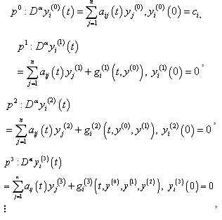
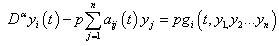
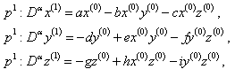
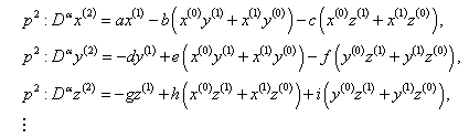
The Homotopy Perturbation Method (HPM), which provides analytically an approximate solution, is applied to various nonlinear problems ([11]-[14]). In this section, we introduce a reliable algorithm to handle the nonlinear ecosystems in a realistic and efficient way. The proposed algorithm will then be used to investigate the system given by:

(1)

subject to the initial condition,

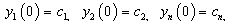(2)

where is a nonlinear function for each .Using the homotopy perturbation method we can construct the following homotopy for ,

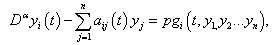(3)

where is the homotopy parameter, which takes values from zero to unity. In case equation (3) becomes a linear equation given by:

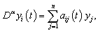(4)

and when p is 1, equation (3) turns out to be the original equation given as system (1). Assuming that the solution of the system (1) is a power series in p given by:

(5)

Substituting equation (5) in equation (3), and equating the terms having identical powers of p, we obtain a series of linear equations in the form:

where the function 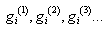satisfy the following equation:

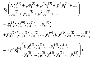Now taking in the equation (5) it gives the solution of the system It is obvious that the above linear equations are easy to solve, and the components of the homotopy perturbation solution can be completely determined as a series solution,

Finally, we approximate the solution 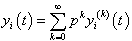by the truncated series

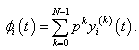(6)

It is also useful, for the system to construct the homotopy, for

(7)

where . In this case, the term is combined with the component and the term is combined with the component and so on. This variation reduces the number of terms in each component and also minimizes the size of calculations. By substituting equation in equation we obtain the following series of linear equations:

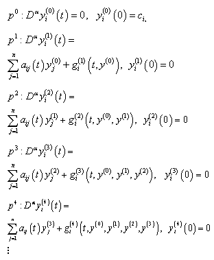
4. Numerical Example

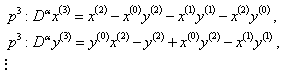
In this section we show the application of the algorithm based on HPM given above to solve four different linear and non linear fractional Ecosystem model.

Example 4.1. Consider the linear system [15]

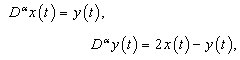(8)

subject to the initial conditions

(9)

We construct the Homotopy

To solve the system given in Eq. we construct the Homotopy as given in Eq. putting Eq. then initial condition in Eq. and then comparing the like powers of we get,

(10)

(11)

(12)

(13)

(14)

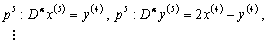(15)

Using the operator , the inverse operator of , on both side of linear equations from with initial conditions we get

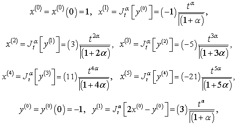
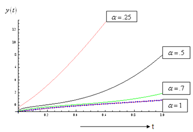
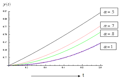
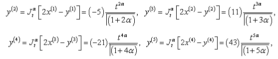The solution of is given by:

the graph of which is given below:

From Fig.1 and Fig.2 we see that the solution obtained by the proposed algorithm for is same as the solution obtained by [16]. Also figures 1 and 2 show the solution for other different values of . Fig 1 and 2 show the solutions in red by HPM of the original system and by HPM of the fractional ecosystem model by blue thick dots.

Example 4.2. Consider the predator – prey system [15].

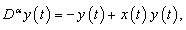(16)

subject with the initial conditions

(17)

We construct the Homotopy

Figure 1. Plot of

Figure 2. Plot of

To solve the system given in Eq. we construct the Homotopy as given in Eq.(7) putting Eq.(5) then intial condition (17) in Eq. (7)and then comparing the like powers of we get,

(18)

(19)

(20)

(21)

Now using the operator , the inverse operator of , on both side of linear equations from with initial condition we get,

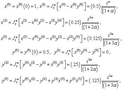hence the solution of is given by

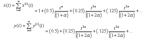This is the accurate and exact solution of the system , [7], using Homotopy Perturbation Method.

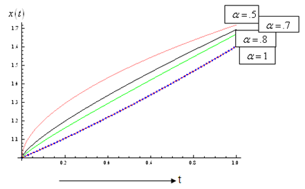Figure 3. Plot of

Figure 4. Plot of

From the Fig.3 and Fig.4 we see that the solution obtained by the proposed algorithm for is same as the solution obtained by [16]. Also fig.3 and 4 show the solution for other different values of .

Figure 3 and 4 show the solutions of HPM to the ecosystem model by red colour and that of the fractional ecosystem model by blue dots.

Example 4.3. Consider the predator – prey system

(22)

where and are constants, subject to the initial conditions

(23)

We construct the Homotopy

To solve the system given in Eq. we construct the Homotopy as given in Eq. putting Eq. then intial condition in Eq. and then comparing the like powers of we get,

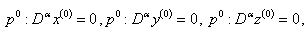(24)

(25)

(26)

Using the operator the inverse operator of on both side of linear equations from with initial condition we get,

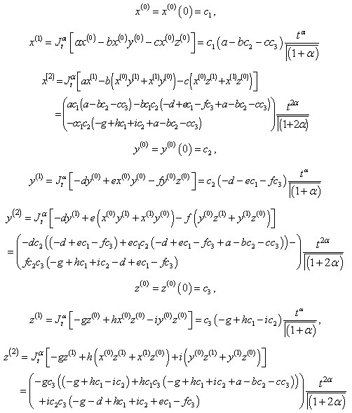Hence the solution is given as

which is the accurate /exact solution of the system using Homotopy Perturbation Method .

Example 4.4. Consider the system [17]

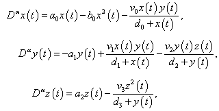(27)

Where are model parameters assuming only positive values , with the initial conditions

(28)

multiplying the first equation of by the factor , the second equation of by the factor 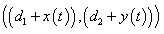and the third equation by the factor To solve the system given in Eq. we construct the Homotopy as given in Eq. putting Eq. then intial condition in Eq. and then comparing the like powers of we get,

(29)

(30)

using the operator the inverse operator of on both side of linear equations from with initial condition we obtained,

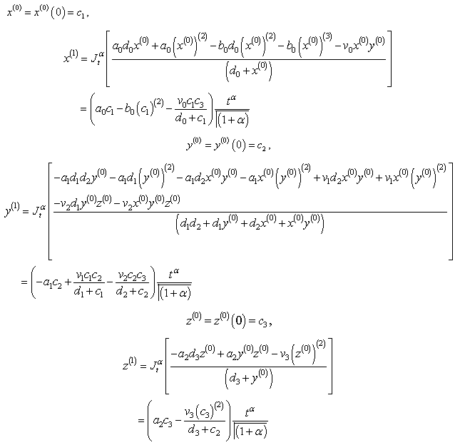Hence the solution is given by

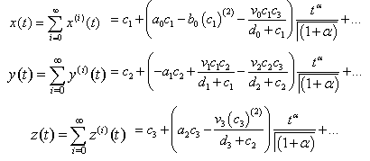This is closed form of solution of the system using HPM.

4. Conclusions

In this paper we have introduced an algorithm based Homotopy Perturbation Method to solve the fractional ecosystem model. The method has been applied to get exact and accurate solution for linear and nonlinear systems of fractional Ecosystem model, the solution obtained matches with the solution of the original ecosystem for α=1 and both the variables (populations) increases with time while value of α decreases and the solution converges to the original solution of the linear and nonlinear ecosystem model as the fractional parameter α tends to 1 as found in two examples. This method can also be applied to similar linear and nonlinear models in other systems. Further it is also verified that the FHPM is more efficient than HPM.

ACKNOWLEDGEMENTS

The first author expresses thanks to fellow scholars, in particular to Rajneesh Kumar, Vipul Kumar Barnwal and Dr. S Das who helped him in preparation of the present paper.