Temesgen Tibebu Mekonnen
Department of Mathematics, Debre Berhan University, Debre Berhan, Post code 445, Ethiopia
Correspondence to: Temesgen Tibebu Mekonnen, Department of Mathematics, Debre Berhan University, Debre Berhan, Post code 445, Ethiopia.
| Email: |  |
Copyright © 2012 Scientific & Academic Publishing. All Rights Reserved.
Abstract
In this paper a generalist predator prey system is modeled as a two dimensional coupled differential system. We identified three vital parameters  stands for the maximum uptake rate of the generalist predator,
  stands for half saturation value and
  such that
  is the conversion efficiency of the generalist predator where
  is the intrinsic growth rate of the predator. Using these parameters a novel way to divide the parameter space based on the number of interior equilibrium solutions admitted by the system has been presented. We investigate the considered model is reach in dynamics and identified various bifurcations that are experienced by the considered system from the parameter space. These are Saddle-Node bifurcation, Trans-Critical bifurcation and pitchfork bifurcation. In this study we offer mathematical proof for the incidence of these bifurcations that take place in the considered dynamical system as the parameters move between the regions presented in the parameter space.
Keywords:
Two Dimensional Differential Systems, Parameter Space, Saddle-Node, Trans-Critical, Pitchfork
Cite this paper: Temesgen Tibebu Mekonnen, Bifurcation Analysis on the Dynamics of a Genralist Predator-Prey System, International Journal of Ecosystem, Vol. 2 No. 3, 2012, pp. 38-43. doi: 10.5923/j.ije.20120203.02.
1. Introduction
A bifurcation is a qualitative change in the behaviour of solutions as one or more parameters are varied. The parametric values at which these changes occur are called bifurcation points. If the qualitative change occurs in a neighbourhood of a fixed point or periodic solution, it is called a local bifurcation. Any other qualitative change that occurs is considered as a global bifurcation[1].The model that is considered in this study was recently studied by[8]. This was examined to study and derive control strategies pertaining to the invasion of leaf mining micro lepidopteron attacking horse chest nut trees in Europe. By choosing specific parameters the authors used graphical analysis to identify the existence of multiple equilibria. Numerical simulations corresponding to a special choice of parameters was closely studied to illustrate the involvement of Hopf bifurcation with unstable limit cycle and Homoclinic bifurcation. But they did not give specific analytical proof and specific identification for the system also experienced Saddle -Node, Trans-Critical and Pitch fork bifurcations. Therefore the work presented in this work extends the study made in[8] by identifying the parameter space for bifurcation diagrams (figures 1-3) and proved analytically their existence. In this paper we investigate the local bifurcations involving the system dynamics. We find that the considered system is very rich in dynamics and involves several interesting bifurcations. A comprehensive analytical bifurcation analysis presented on the local bifurcations: Saddle Node, Trans- critical and Pitchfork bifurcations. Along with the local bifurcations the author also investigated the Bogdanov- Takens (codimension 2) and global bifurcations in which the detail analysis is in progress.Division of the parameter space as shown in figures 3, 4 and 5 with respective parameter values η = 1, η > 1 and η < 1 are the fundamental bifurcation diagrams of this study. In the next section we present the basic concepts, the model, steady state solutions and division of parameter space in the system dynamics. In section three, the central part of this study: the bifurcation analysis is analysed. Conclusions are presented in section four.
2. The Model, Steady State Solutions and Division of Parameter Space
2.1. The Model
Let X and Y represent the density of Prey and Generalist Predator respectively with the assumption that each species grow logistically in the absence of the other. Further we assume that the predator’s functional response is of Holling type II and hence the dynamics of the considered system is  | (1) |
 | (2) |
The constants a (d), k1 (k2) are the intrinsic growth rate and carrying capacity of prey (predator). b, c stands for maximum uptake rate and half saturation value of the predator and e = δb (0 < δ < 1) where δ is the conversion efficiency. From the above model we clearly observe that the predator can survive in the absence of the prey and the per capita growth rate of the predator is enhanced by  in the presence of prey. To reduce the number of parameters we non-dimensionalise the considered model (1, 2) and obtain the following:
 | (3) |
 | (4) |
Where  | (5) |
With
2.2. Nature of Steady State Solutions
In this section we study the existence of equilibrium solutions of (3, 4) and study their nature through linear analysis. Clearly the system admits (0, 0) as trivial equilibrium and (1, 0), (0, 1) to be its axial equilibrium points. The interior equilibrium points are the intersection points of the isoclines y=g(x) and y=h(x) in the interior of the positive quadrant. Following the standard linear analysis it is easy to observe that (0, 0) and (1, 0) are unstable node and saddle point respectively. We observe that the nature of (0, 1) depends on the values of the parameters α and θ. If θ / α ≤ 1 then (0, 1) is stable and it becomes a saddle if θ / α > 1. In the latter case (0, 1) is unstable in the x-direction and stable in the y-direction. Thus we have the equilibria (0, 0), (1, 0) to be always hyperbolic. Where as (0, 1) is hyperbolic when α ≠ θ and it turns to non hyperbolic when α equals θ. Analysing the Jacobian of the system (3, 4) at its interior equilibrium point (x*,y*) gives the associated characteristic equation to be To understand the nature of an interior equilibrium solution of the system (3, 4) we need to study the signs of the trace
  and the determinant
  which are respectively the sum and product of the Eigen values of the considered Jacobian matrix[2].
2.3. Division of Parameter Space
From the qualitative behaviour of the isoclines of the system (3, 4) we can observe that there is a possibility for the system to admit multiple interior equilibrium solutions. The number of interior equilibrium solutions admitted by the considered system (3, 4) and its dependence on the involved parameters can be best understood by analysing the following cubic equation | (6) |
This is obtained by equating the functions g(x) and h(x) (5). If x is a positive root of (5) then either (x, g(x)) or (x, h(x)) gives an interior equilibrium point of the system (3, 4). Thus the number of positive roots of (5) corresponds to the number of interior equilibrium solutions admitted by the system (3, 4). Hence from this cubic polynomial equation we observe that the system (3, 4) admits a maximum of three interior equilibria in the first quadrant of the phase space. The discriminant of the cubic polynomial equation (6) is  | (7) |
The sign of ∆P determines the number of real roots admitted by (6). If ∆P is either < 0, = 0 or > 0 then P(x)=0 admits three distinct real roots, three real roots with one of them repeated twice or three roots with one of them real respectively[6]. For a chosen set of parameters α, θ and η sign of the discriminant along with the signs of the coefficients of the equation P(x) yield further information on the roots of the equation (6). For the sake of simplicity let us denote the constant term in (6) by  | (8) |
This represents the product of the roots of (6). Analyzing the curves ∆P =0 and  it can be verified that
  is tangential to ∆P =0 at
  which is denoted by c and these two curves intersect at
  denoted by e (figures 2 and 3). From these figures we observe that there is another significant point lying on the curve ∆P=0 denoted by f at which the curve takes a sharp turn. It is further observed that this point f also satisfies the equations
 | (9) |
 | (10) |
Implying that the equation (6) admits a triple root at f[6]. It is interesting to note that the points c and e merge in f when η = 1. It can be observed that, depending on the value of the parameter (η=1,η>1 or η<1), the equations ∆P=0 and  divide the positive quadrant of the
  space into several significant regions as given below.If η = 1 the positive quadrant of the
  space is divided into four regions (Figure 1) given byRegion I =
  Region II =
  Region III =
  Region IV =
  If η>1 then region I is further divided into Region Ia =
  Region Ib =
  And regions II, III and IV remain as in the case η = 1 .(Figure 2)
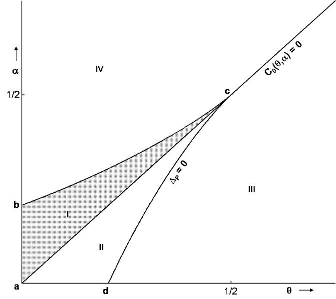 | Figure 1. this figure represents division of the parameter space for η= 1. The regions bounded by  and ∆P=0 enclosed by {a,b,c} and {a,c,d} represent regions I and II respectively. Regions lying below (above) the line and ∆P=0 enclosed by {a,b,c} and {a,c,d} represent regions I and II respectively. Regions lying below (above) the line  is Region III(IV). The system admits two interior equilibrium points in the region I, one interior equilibrium point in Regions II & III and no interior equilibrium point in region IV is Region III(IV). The system admits two interior equilibrium points in the region I, one interior equilibrium point in Regions II & III and no interior equilibrium point in region IV |
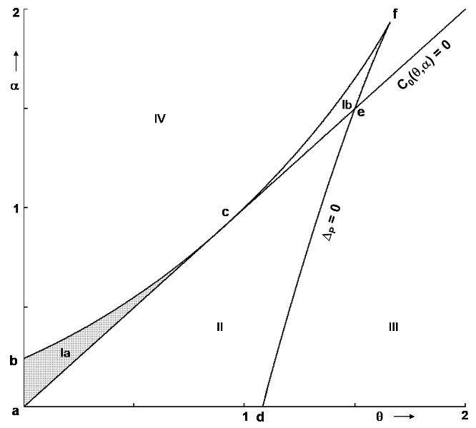 | Figure 2. this figure represents division of the parameter space for η > 1. The regions bounded by  and ∆P=0 enclosed by {a,b,c}, {c,f,e} and {a,d,e} represents regions Ia, Ib and II respectively. Region lying below (above) the line and ∆P=0 enclosed by {a,b,c}, {c,f,e} and {a,d,e} represents regions Ia, Ib and II respectively. Region lying below (above) the line  is region III(Iv) for η = 9 (a representative for η> 1). The system admits two interior equilibrium points in the region Ia, one interior equilibrium point in regions II & III and no interior equilibrium point in regions Ib & IV is region III(Iv) for η = 9 (a representative for η> 1). The system admits two interior equilibrium points in the region Ia, one interior equilibrium point in regions II & III and no interior equilibrium point in regions Ib & IV |
On the other hand if 0<η<1 then region II is divided intoRegion IIa =  Region IIb =
  And the regions II, III and IV remain as in the case η= 1. (Figure 3)
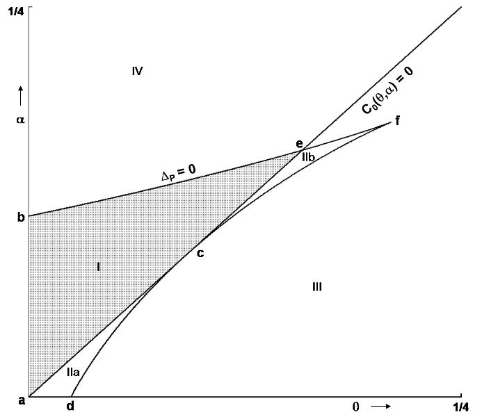 | Figure 3. this figure represents division of the parameter space for 0< η < 1. The regions bounded by  and ∆P=0 enclosed by {a,b,e}, {a,c,d} and {c,e,f} represents regions I, IIa and IIb respectively. Region lying below (above) the line and ∆P=0 enclosed by {a,b,e}, {a,c,d} and {c,e,f} represents regions I, IIa and IIb respectively. Region lying below (above) the line  is region III(Iv) for η=0.1 (a representative for 0 <η < 1). The system admits three interior equilibrium points in the region IIb, two interior equilibrium points in region I and no interior equilibrium point in regions IV is region III(Iv) for η=0.1 (a representative for 0 <η < 1). The system admits three interior equilibrium points in the region IIb, two interior equilibrium points in region I and no interior equilibrium point in regions IV |
From the nature of the boundary equilibrium solutions we observe that (0, 1) changes its stability nature as the parameter cross the curve  indicating occurrence of bifurcation along the curve
  . Similarly we also observe change in the number of equilibrium solutions of the system as the parameter cross the discriminant curve ∆P=0 presenting another incidence of bifurcation. This curve also contains three significant points’ c, e and f. In the next section we study the significance of these curves and the importance of the points mentioned above.
3. Bifurcation Analysis
Division of the parameter space as shown in figures 1, 2 and 3enables us to recognize some basic bifurcations associated with the system as the parameters move from one region to another. The following discussion highlights the significance of various segments and points that are presented in the above figures and we present the local bifurcations occurring in the considered system.Theorem1. (Saddle-Node Bifurcation) Let  be an interior equilibrium point of the system (3, 4). If the parameters α, θ, and η corresponding to this equilibrium satisfy ∆P=0 and
 , then the system experiences a saddle-Node bifurcation except when
  Proof: let’s represent the dynamical system (3, 4) by a vector form given by
  | (11) |
Let  be an interior equilibrium point of the system (3, 4). Clearly we have
  to be a root of
  i.e.
i.e.  and also
  (due to monotonicity property of the y isocline). Since a saddle node bifurcation takes place at an equilibrium point (x*,y*) if the Jacobian matrix J(x*,y*) of the given system at the equilibrium point (x*,y*) has simple zero Eigen value, therefore, first we find conditions under which the Jacobian matrix J(x*,y*) has simple zero Eigen value. These conditions are both the determinant denoted by DetJ(x*,y*) and trace denoted by TrJ(x*,y*) of the Jacobian matrix J(x*,y*) is zero[4]. The Jacobian matrix at an interior point
  of the system (3, 4) is given by
 | (12) |
We have  | (13) |
Thus DetJ(x,y)=0 implies that | (14) |
And we have assumed that  which is the sum of the Eigen values of the Jacobian matrix (12). Therefore condition (14) ensures that the Jacobian matrix J(x,y) has simple zero Eigen value. Observe that the condition (14) is nothing but the equation
  Thus if an interior equilibrium (x,y) of the system (3, 4) satisfies (14) then its x component is a double root of P(x)=0. In which case, the corresponding parameter values α, θ, and η of x satisfy the discriminant equation ∆P=0 (6). We shall use the Sotomayor theorem[3] to establish the existence of Saddle-Node bifurcation. Below we shall compute all the terms that are necessary to verify the Sotomayor theorem. Under the assumption (14) the Jacobian matrix J(x,y) takes the form
 Let
Let  be a non hyperbolic interior equilibrium point of (3, 4). Taking the scalar α as a bifurcation parameter and solving for α from the prey and predator zero growth isoclines (3, 4), we have
  | (15) |
Denoting  by
by  and using (15) we obtain
 | (16) |
Let  Be an Eigen vector of
  corresponding to the Eigen value λ=0. Thus v1 and v2 satisfy the simultaneous equations
 | (17) |
 | (18) |
After performing standard computation of the Eigen vectors and choosing an arbitrary Eigen vector v2=1 we obtain | (19) |
Now let  be an Eigen vector of
  | (20) |
Corresponding to the Eigen value λ=0, thus using similar computation of the Eigen vector W and choosing an arbitrary vector w2=1 we obtain | (21) |
Of the matrix  corresponding to the Eigen value λ=0. Differentiating the vector function
  (11) with respect to the bifurcation parameter α we obtain
 Hence we have
  | (22) |
Since y is always greater than unity (monotonocity of predator zero growth isocline)  is always positive. Now we examine the nature of the expression
  where
where  is an Eigen vector (19). The expression
  is defined in[3,7] by
 | (23) |
Competing each term of the right hand side of (23) we obtain Therefore we have
 | (24) |
From (14) we observe that the right hand side of (24) is different from zero if  . If
. If  , we have the corresponding value for
  which is the predator zero growth isocline. Thus (22) and (24) satisfies the conditions for Saddle-Node bifurcation in the Sotomayor Theorem[3] and we observe that the system (3, 4) experiences Saddle-Node bifurcation at an equilibrium point
  if the parameters α, η and θ satisfy ∆P=0 except when
 | (25) |
From figures 1-3 we observe that  which is the line
  corresponds to a state where an interior equilibrium point collides with the axial equilibrium (0, 1) resulting in Trans-Critical bifurcation. Thus we have the following resultTheorem2. (Trans-Critical Bifurcation) If
  then the system (3, 4) experiences Trans-Critical bifurcation at (0, 1) whenever the parameters α, θ and η are positive and satisfy the equation
  except when
  .Proof: Let us consider (12) which is the Jacobian of system (3, 4) evaluated at an equilibrium point (x, y) given by
 Since the equilibrium point of study is (0, 1), evaluating the Jacobian matrix A(x,y) at (0, 1) we obtain
 Here observe that the matrix B has a single zero Eigen value as its determinant is zero and we assumed that the trace
  . This ensures that the Jacobian matrix B has simple zero Eigen value. We shall establish the existence of Trans-Critical bifurcation at the equilibrium (0, 1) of system (3, 4) by using Sotomayor theorem[3]. Below we compute all the needed terms to verify the conditions for existence of Trans-Critical bifurcation at (0, 1). Let
  be an Eigen vector of the matrix B corresponding to the Eigen value λ=0. Hence using the standard computation of the Eigen vector and choosing an arbitrary vector v1=1 we obtain
 | (26) |
Now let  be an Eigen vector of the matrix
 Differentiating the vector function
  (11) with respect to the bifurcation parameter
  and evaluating at the point (0, 1) we obtain
 And hence
  | (27) |
The expression  defined in[3] as
 Evaluating
  at (x, y) = (0, 1) and using (26) we obtain
 And hence we have
 | (28) |
Now let us consider the expansion of the term  which is given by[3] by
 Evaluating this at point (0, 1) and using (26) along
  we obtain
  And hence we have
 | (29) |
Observe that the RHS of (29) is different from zero for  Therefore Sotomayor theorem[3] together with equations (27), (28) and (29) imply that the system (3, 4) experiences Trans-Critical bifurcation at (0, 1) which occurs on the curve
  in the
  space for any positive θ except at
  From the above discussion we observe that the parameters belonging to the set
  These are candidates for points of codimension 1 bifurcation and for
  the points in the set
  Which is nothing but the set of points {e, c, f} are candidates for codimension 2 bifurcation while for the case η=1 the points c=e=f is a candidate for codimension 3 bifurcation. Thus we have a result in which Pitchfork bifurcation exists at the point
  which is one of the codimension 2 bifurcations. (Work is in progress on results where Bogdanov-Takens (codimension 2) bifurcation exists at the point e. And then for the parametric value η=1 at the point c=e=f we have also investigated a Degenerate Bogdanov-Takens (codimension 3) bifurcation.)Theorem3. (Pitchfork Bifurcation)If
  then the system (3, 4) experiences Pitchfork bifurcation at the intersection point
  of the two curves
  and ∆P=0 for all parametric values η>1Proof: To prove this theorem we make use of the Sotomayor theorem[3] which involves four conditions. The first three conditions follow from the equations (27), (28) and (29) evaluated at
  Below we shall establish the validity of the fourth condition. For a function f(x,y,z) defined in[3,5] we have
 Evaluating at (x, y) = (0, 1) and using (26) we obtain
 Therefore
  | (30) |
Observe that the right hand side of (30) is different from zero for all parametric valuesη>0, therefore using the equations (27), (28), (29) and (30) evaluated at  for η>0 in Sotomayor theorem[3] we infer that the system (3, 4) experiences a Pitchfork bifurcation at (0, 1) on the curve
  in the
  space.
4. Conclusions
In this study we offer mathematical proof for the incidence of various bifurcations that take place in the considered dynamical system as the parameters move between the regions presented in the parameter space as shown in figures 1-3. The identified bifurcations included Saddle-Node, Trans-Critical and Pitchfork bifurcations. The Saddle-Node bifurcation takes place along the curve ∆P=0 except when at the cusp point f. The Trans-Critical bifurcation of the system occurred at the equilibrium point (0, 1) as the parameters θ and α move along the curve  (figures 1-3) in the interior of positive quadrant of
  space for any positive η and the system experiences the Pitchfork bifurcation when the parameters θ and α are at the point c for any positive
  We also investigate the occurrence of Bogdanov-Takens (codimension 2) bifurcation at the point e and the detail study is in progress. Further analysis can be done to identify the global behavior of the system at the point f. At this juncture we wish to mention that we could not identify the type of bifurcation that can take place at the point where c, e and f coincide whenη=1. We intend to pay more attention to this at a later stage.
ACKNOWLEDGEMENTS
I would like to express my sincere gratitude to Dr. P.D.N. Srinivasu, Professor of Mathematics for his willingness to see and comment all my works, his many valuable suggestions, encouragement and constant support in doing this work. I also forward my gratitude to Dr. B.S.R.V.Prasad and Dr.Kiran Kumar for their constant help to complete this work.
References
| [1] | Ali Nayfeh, Nonlinear Dynamical Systems and Chaos, Prentice Hall, Englewood Cli_s, 1983. |
| [2] | George F.Simmons, 1972, Differential Equations, McGraw- HILL PUBLISHING COMPANY LTD, New Delhi. |
| [3] | Lawrence Perko, 2001, Differential Equations and Dynamical Systems, Third Edition, Springer, New York. Online Available: http://journal.sapub.org/ajb. |
| [4] | Nils Berglund, 2001, Perturbation theory of Dynamical Systems, Switherland. |
| [5] | S.M. Nikolsky, 1977, A Course of Mathematical Analysis, Volume 1, MIR Publishers, Moscow. |
| [6] | Turnbull, H.W., 1952, Theory of equations, Intercience publishers Inc, New York. |
| [7] | Walter Rudin, 1976, Principles of Mathematical Analysis, McGraw-HILL International Editions, Third Edition. |
| [8] | Magal.C, Cosner.C and Ruan.S; 2008, Control of Invasive Hosts by Generalist Parasitoids. Mathematical Medicine and Biology, 25, 1-20 |
 Abstract
 Reference
 Full-Text PDF
 Full-text HTML