1. Introduction

A problem of global warming due to the greenhouse effect appeared at the end of the 20th century and till now it is a serious environmental issue. Global warming is defined as the warming of the Earth by greenhouse gases emitted into the atmosphere naturally or through human activities. The greenhouse effect as the process by which some of outgoing radiative energy is transferred back to the surface and heats the Earth, was discovered by Joseph Fourier in 1824, and first investigated quantitatively by Svante Arrhenius in 1896[1]. Gases that trap heat in the atmosphere are often called greenhouse gases. The primary greenhouse gases in the Earth atmosphere are water vapor, carbon dioxide, methane, nitrous oxide, and ozone[2]. When these gases are ranked by their contribution to the greenhouse effect, the most important are:

Carbon dioxide is released into the atmosphere by the burning of solid waste, woods and woods products, and fossil fuels (oil, natural gas, and coal). Nitrous oxide emissions occur during various agricultural and industrial processes, and when solid waste or fossil fuels are burned. Methane is emitted when organic waste decomposes whether in landfills or in connection with livestock farming. Methane emissions also occur during the production and transport of fossil fuels. In addition to the main greenhouse gases listed above, other greenhouse gases include hydrofluorocarbons (HFCs), perfluorocar bons (PFCs), and sulfur hexafluoride (SF6). All of them result exclusively from human industrial activities.

The greenhouse gases greatly affect the temperature of the Earth; without them, the Earth surface would be on the average about 33 °C colder than at present[3]. The Fourth Assessment Report of the Intergovernmental Panel on Climate Change (IPCC) in 2007 concluded that we can say with high confidence that the effect of human industrial activities since 1750 has warmed the planet. It also says that the observed temperature very likely that increases since the middle of the twentieth century.

Table 1. The Primary Greenhouse Gases in the Earth Atmosphere Gas Element Symbols Contribution (%) Water Vapor H2O 36 -72 Carbon Dioxide CO2 9 - 26 Methane CH4 4 - 9 Ozone O3 3 - 7

Among all greenhouse gases, carbon dioxide emission is the most important cause of global warming. Since the beginning of the Industrial revolution, the burning of fossil fuels has contributed to the increase in carbon dioxide in the atmosphere from 280 ppm (parts per million) to 380 ppm[4]. The emissions of CO₂ have dramatically increased within the last 50 years. Recent investigations have shown that inconceivable catastrophic changes in the environment will take place if the global temperatures increase by more than 2° C. This value corresponds to a carbon dioxide concentration by about 450 ppm in the atmosphere. As the content raises on average 2 - 3 ppm each year, the critical value will be reached in approximately 20 to 30 years from now.

The Fourth Assessment Report predicts that global temperatures could rise from something between 1.1° C to 6.4° C by the end of the 21st century. It is very likely that hot extremes, heat waves, and heavy precipitation events will continue to become more frequent. By the second half of the 21st century, wintertime precipitation in the northern mid to high latitudes and Antarctica will rise. At the same time, Australia, Central America and Southern Africa are likely to see decreases in winter precipitation. The findings of the 2007 IPCC report reinforced the widespread consensus that action is required quickly to stabilize the atmospheric greenhouse gas concentrations. According to Nicholas Stern report[5] the economic cost of global warming stabilization would be about one per cent of world GDP. This implies that the constant long-term monitoring of the contents of carbonic acid in the atmosphere is one of major tasks of the complex program for stabilization of a climate.

2. Methods of Investigations of the CO₂ Content

The first measurements of the composition of the air were carried out using chemical methods at the end of the 18th century. It was established that the main components of the Earth atmosphere are oxygen, nitrogen, and carbon dioxide. More precise data on the air composition were subsequently obtained, using the physicochemical methods of chromatography[6] and mass spectrometry[7]. Enhancing the accuracy of the old methods and developing new methods made it possible to detect such subtle effects as diurnal, seasonal, and multiyear variations in the minor constituents (CO, SO₂, NO₂, NO, O₃, etc.) of the atmosphere. The sampling method representative of background conditions may still contain useful information. The data selection methods are able to obtain the values from which monthly and annual means are calculated. These methods are used by the Air Resources Laboratory of the National Oceanic and Atmospheric Administration (NOAA). In the mid-1970-s four baseline monitoring stations were established to conduct continuous measurements of atmospheric mixing ratios, including CO₂. The stations are operated by NOAA's Climate Monitoring and Diagnostics laboratory (CMDL) at: Point Barrow, Alaska; Cape Matatula, American Samoa; Mauna Loa, Hawaii; and South Pole, Antarctica. All these stations are situated far from big cities and industrial centres.

Obviously, for acceptance of adequate measures on stabilization of the climate it is also necessary to supervise sources of emissions of carbonic gas in large cities and industrial centres. However, here the high-precision gas analyzers for measurement of concentration of carbonic acid are unsuitable, as the data in question are greatly affected by the presence or absence of nearby local sources of emissions: factories, power stations, transport routes, etc. In order to obtain representative data characterizing the overall situation in some industrial region, an averaging period of about one month is necessary[8]. This is why the most practical and suitable means of investigating such variations is the astrophysical method[9], as it allows us receiving total amount of molecules of carbonic gas at once over the full depth of the Earth atmosphere.

The essence of the method consists in comparing the computed and observed profiles of the absorption lines for a given component of the air. The observed in the spectrum of the Sun telluric line profiles are recorded with the help of a solar telescope and spectrograph of sufficiently high resolving power. Then one should calculate the line absorption coefficient and solve the equation of transfer for line radiation over the full depth of the atmosphere. It is necessary to make these calculations for concrete physical conditions in the atmosphere at the moment of observations. As a result of comparison of observed and theoretically computed line profiles it is possible to receive the content of a given component of the air at once on the full thickness of the Earth atmosphere.

According to[10] and[11], the technogenous emissions of carbon dioxide produce very significant spatial and temporal heterogeneities of the CO₂ content in the layer 350-500 m above the ground, the greatest heterogeneities being in the lower 50-meter layer. Here, under unfavourable meteorological conditions, spatial variations of man-made emissions may reach 10% of the background. Even greater variations as high as 15% are associated with the diurnal and seasonal cycles of intensity of the anthropogenous emissions.

To search the influence of these variations on the recorded equivalent widths of the CO₂ lines, we calculated the contribution of the lower 500-meter layer into the full equivalent width of a line using CIRA-1961 model of the Earth atmosphere[12]. It turned out, that no more 9 % of full equivalent width of a line are formed in this layer. It means that uncertainties of the registered equivalent widths of the CO₂ lines caused by spatially-time variations of the CO₂ content in the lower 500-meter layer do not exceed 1.5%. It is a small value in comparison with a random error of about 5% in our observations. Thus, it is to be hoped that the astrophysical method will be an effective tool for purposes of ecological monitoring.

For obtaining authentic data about long-term variations CO₂ in the Earth atmosphere it is necessary to get records of the spectrum of the Sun strictly under the same conditions. An invariance of the parameters of a telescope, spectrograph and recording equipment can be supervised. But identity of physical conditions in the atmosphere (temperature, pressure and humidity of air, the speed and direction of a wind) cannot be achieved. Hence, it is necessary to search the influence of these parameters on the observed profiles of CO₂ lines.

3. Monitoring of the Oxygen Content

As the content of oxygen in the atmosphere may be accepted as constant[13], this circumstance can be used for the control of invariance of parameters of a telescope, spectrograph and recording equipment during several years. In Figure 1 diagram of dependence of equivalent width W of the oxygen line λ6295.178 Å from atmospheric mass M (curve of growth) is presented: points indicate values obtained on 4 and 5 August 1970, crosses pertain to 3 May and 27 December 1990. Note that the data for 3 May and 27 December 1990 were reduced to the physical conditions of 4-5 August 1970 (details see in[13]).

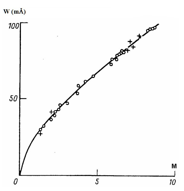Figure 1. Dependence of equivalent width W of the the oxygen line λ6295.178 Å on atmospheric mass M (curve of growth)

Inspection of the Figure 1 shows that deviations of individual observations from the average curve, constructed using the r.m.sq. method, do not exceed 1%. Thus it can be concluded that for the last 20 years parameters of the telescope, spectrograph and recording equipment have remained constant to within about 5%.

4. Variations of the Carbon Dioxide Content

4.1. Choice of Suitable Lines CO₂

The electronic bands of the CO₂ molecule are located in the ultraviolet, near λ1750 Å, and thus are inaccessible to ground-based observations. The vibration-rotation bands cover a considerable part of the spectrum from λ7600 Å to λ150,000 Å[14]. An analysis of the profiles of the CO₂ lines, based on the tables in[15] and the Photometric Atlas in[16], enabled us to select two weak individual lines with "clean" (not blended by telluric and Fraunhofer lines) profiles in the λ20,800 Å region: the lines λ20,756.11 Å and λ20,758.51 Å. Unfortunately, in this region there is also a large number of irregularly spaced absorption lines due to water vapor[15]. Hence it is possible that CO₂ lines selected by us can be blended with weak telluric lines of water vapor. Figure 2 shows a strip of the spectrum in the λ20,800 Å regions. Here the solid line is a spectrum found for a humidity of air of 76 %, and dashed line is the spectrum for a humidity of 23 %. From Figure 2 it follows that in the considered region there is one very strong line of water (line number 1) and some weak lines (0, 4, 5 and 8). It is obvious that CO₂ lines λ20,756.11 Å (marked by 7) and λ20,758.51 Å (marked by 6) are not blended by lines of water vapor.

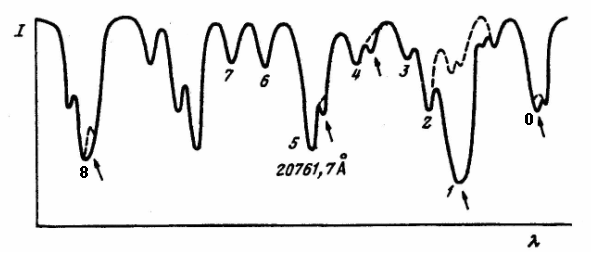Figure 2. Solar spectrum in the λ20,800 Å region. Solid line: humidity 76 %, dashed line: humidity 23 % (I – intensity, λ - wavelength)

4.2. Seasonal Variations of the Carbon Dioxide Content

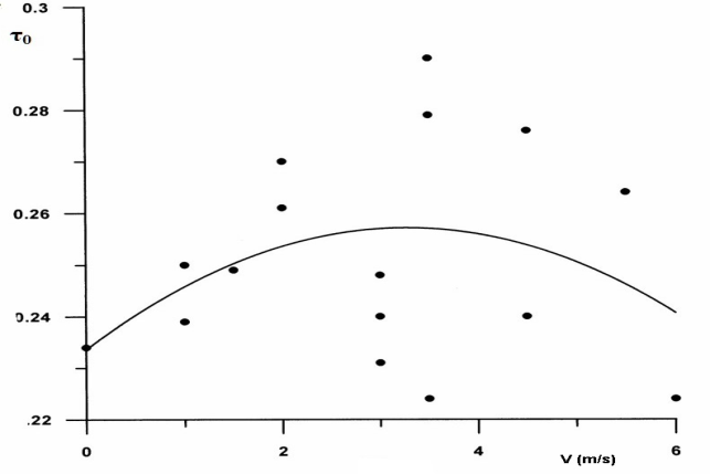
A question on seasonal changes of CO₂ concentration in the atmosphere is of great importance for obtaining reliable data on long-term changes of carbonic acid. According to[10], in many cities of the world the seasonal run of CO₂ content is well expressed. Usually it has a minimum at the end of summer and a maximum in winter months. Apparently it occurs due to seasonal prevalence of photosynthetic activity of plants in summer and with growth of anthropogenous emissions in cities in the winter period as a result of an increase in the consumption of fuel at heating of buildings. However, appreciable deviations from this "typical" course are marked. For example, the minimum of СO₂ concentration in Berlin falls on December, while in Teheran on June. The reasons of it can be features of local seasonal productivity of anthropogenous sources and geographical location of a city.

We have executed researches of seasonal variations of carbon dioxide content in Moscow air basin using data of the observations obtained from February to November during 1992 - 1995. In Figure 3 the seasonal run of the optical depth τ₀ in the centre of CO₂ lines is presented. According to[13], τ₀ is proportional to the number of CO₂ molecules in all thickness of the atmosphere.

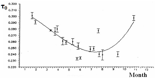Figure 3. The seasonal run of the optical depth τ0 in the centre of CO2 lines (points are the results of observations, continuous line is the approximating polynomial of the 3rd degree)

From Figure 3 it follows that the number of CO₂ molecules in all thickness of the atmosphere reach the minimal value at the end of July - beginning of August and grow in winter (with a maximum presumably since November till February). Nearly the same results were obtained by a local method on Monte Cimone, Italy (height of 2165 m above the sea level) and in the City of Cold Bay, Alaska[17].

The significant (about 20 %) seasonal variations of CO₂ content found out by us in an atmosphere of Moscow put a question about their correct account at researches of long-term changes. However, it is possible to avoid this difficult procedure if to make observations from the end of July till the beginning of September.

4.3. A Wind and Variations of the CO₂ Content

Regular measurements of the CO₂ concentration by local methods in ground layers of the atmosphere in suburbs have shown that the CO₂ content grows when wind blows from the city or from the direction of powerful anthropogenous sources. A high concentration is observed also, as a rule, at a weak wind[18, 19].

Since our telescope is located within the city boundaries, about 8 km to the south from its centre, the wind direction can affect the results of observations. For research of probable dependence of CO₂ content on the direction of wind we have selected observations during February - November of 1992-1995. Despite considerable dispersion of points in Figure 4, it is possible to draw a conclusion that the weak dependence of measured CO₂ concentration from the direction of wind is traced: for the southern wind it decreases a little and for the northern wind (from the centre of Moscow) it grows.

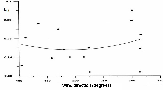Figure 4. Dependence of the optical depth τ0 in the centre of CO2 lines on the wind direction (azimuth A = 0 ° corresponds to the north, A = 90 ° - to the east, A = 180 ° - to the south and A = 270 ° - to the West. The dots are observation results, solid line is a r.m.sq approximation.

We carried out also special researches of the dependence of the CO₂ concentration on the wind speed in the range from 0 up to 6 m/s. As Figure 5 shows, for a wind speed of about 3 - 4 m/s a weak maximum is observed.

Figure 5. The optical depth τ0 in the centre of CO2 lines versus wind speed v. The dots: observations results, solid line: r.m.sq approximation

4.4. Long-Term Variations of the Carbon Dioxide Content

Our first set of data of the carbon dioxide content in the air basin above Moscow were obtained on 3 December 1969 for an atmospheric mass M = 4.86 and an air temperature T = 272.8 К (-0.2°С). An average of the equivalent widths for the two lines was 252 ± 4 mÅ.

The second set of the data was obtained on 27 September 1991 for atmospheric masses M from 1.88 to 12.00 at T = 292 К (19°С). The equivalent widths of the lines are plotted against the atmospheric mass in Figure 6.

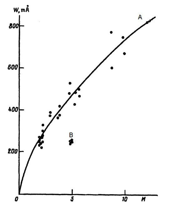Figure 6. Dependence of equivalent width W of the CO2 lines λ20,756.11Å and λ20,758.51 Å on atmospheric mass M (curve of growth). A: 27 September 1991 (the dots: observation results, solid line: r.m.sq approximation); B: observation results for 3 December 1969.

For M = 4.86 (as in case of the first set of the data) our graph gives an equivalent width (averaged over the two lines) W = 476 ± 2 mÅ, which is significantly higher than the value W = 252 ± 4 mÅ for 3 December 1969.

To obtain from these data the actual variation in the CO₂ content of the atmosphere, we have to eliminate seasonal variations of the line widths due to variations in the air temperature, air density, and photosynthesis. The results in[13] indicate that these CO₂ lines can be considered as "weak." In this case the equivalent width can be expressed as a function of the temperature T and the total number N of CO₂ molecules in the line of sight directed to the Sun:

W = (aN/T) exp (- hcF/kT), (1)

where N is the total number of CO₂ molecules on the line of sight, F is the energy of the lower level of the line in cm^-1, a is a constant factor (other notation standard). According to[16], for the first line F = 719 cm^-1, and for the second F = 719 cm^-1.

To calculate the variation of the equivalent width due to the temperature increase from 272.8 К on 3 December 1969 to 292 К on 27 September 1991, we substituted into (1) the temperature at the effective height of formation of the weak lines, which, according to[13], is 6 km. Using the atmospheric model from[12], we found that the difference of temperatures between a height of 6 km and the sea level is 42 K, while the temperature difference from season to season is about the same at 6 km and at the sea level. Thus, for the calculations we took T = 231 К on 3 December 1969 at h = 6 km and T = 250 К on 27 December 1991 at the same altitude. This enhances the first CO₂ line by a factor of 1.303, and the second line by a factor of 1.297, giving an average increase by a factor of 1.3. Consequently, taking W = 252 ± 4 mÅ for 3 December 1969 as the initial value, we get for 27 September 1991 an equivalent width W = 328 ± 4 mÅ due to the increase in the air temperature by 19 K.

The next most important seasonal effect influencing the equivalent width of the CO₂ lines is the summer drop in the CO₂ content associated with the summer photosynthesis maximum in the forests at northern midlatitudes. These variations can have an amplitude of up to 1.5%[20].

Finally the change from winter to summer is accompanied by a reduction in the equivalent widths of the telluric lines due to the additional drop in the air density by approximately 0.5%[13]

Thus the "theoretical" value W_T for 27 September 1991 is found from W by reducing the latter by 2%, to give W_T = 322 ± 4 mÅ. The observed value for this date W = 476 ± 5 mÅ. This means that the equivalent width of the CO₂ lines increased by 154 mÅ, or 48%. According to (1), one may conclude that the CO₂ content in the air basin of Moscow has grown by about 48% from December 1969 to September 1991. It is necessary to pay attention that the growth in the concentration of carbonic acid at the climatic observatory Mauna Loa for the period since 1973 on 1991 was about 8 %[21].

The found by us in 1992[22] fact of a significant excess of the CO₂ content over the city in comparison with the suburb was confirmed 5 years later by Idso et al.[23]. They carried out measurements of CO₂ concentration in the suburb and across the Phoenix city (Arizona, USA) at heights from 2 m up to 1.6 km. The performed observations have shown that in the atmosphere of the city, the CO₂ concentration is approximately 1.5 times higher in comparison with the suburb.

In 1998 - 1999 we have obtained new records of CO₂ lines λ20,758.51 Å and λ20,756.11 Å on the ATB-1 solar telescope (Moscow). To exclude a possible influence of the morning temperature inversions on the results found by us earlier[24], we carried out our observations only near the midday. Besides, the observations were carried out only at the end of summer and in the early autumn when physical conditions in the atmosphere are close to the "average atmosphere"[12]. It reduces the errors of calculations due to the account of seasonal variations. Results of processing of the observations have shown that a steep rise in the abundance of carbonic acid in the air basin of Moscow started from the beginning of 1990s, and to the end of 1999 the CO₂ content exceeded the level of 1969 2.5 times[25]. During the same period, at points distant from big cities and industrial centres (“rural"-type sites), growth in the carbonic acid quantity has been only approximately 11 %[21].

In September 2003, October 2005 and September 2007 monitoring of carbonic acid in the Moscow air basin continued. Using new data and results of all previous observations, we have obtained the run of the СO₂ abundance in the atmosphere of Moscow for 38 years, presented in Figure 7 by curve I. For comparison, results of CO₂ long-term monitoring in so-called "rural" type atmosphere[21] are shown by curve II. Curve III shows the growth of the vehicles quantity N (in Millions) in Moscow from 1969 for 2007.

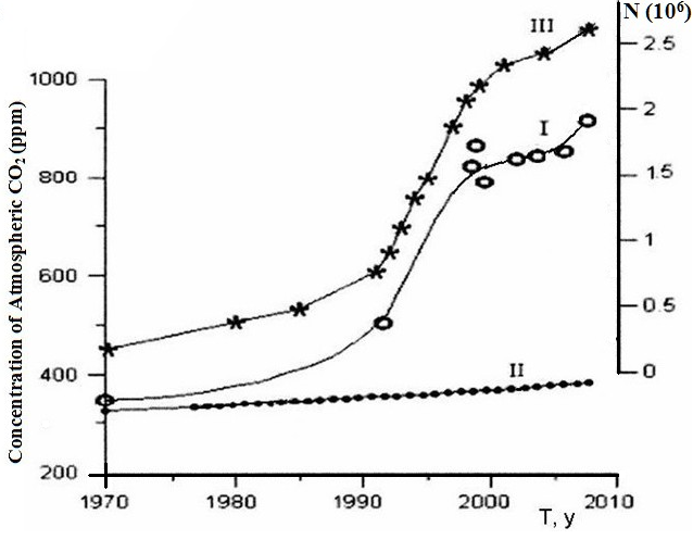Figure 7. Long-term variations of the CO2 content (I: observation results in Moscow air basin; II: “rural" type atmosphere[21]); III: growth of amount of vehicles in Moscow from 1969 till 2007

As can be seen from Figure 7 the rate of the growth of CO₂ concentration in the atmosphere above Moscow considerably exceeds the corresponding values for NOAA CMDL Baseline Observatories: Barrow (Alaska), Mauna Loa (Hawaii), American Samoa and the South Pole, according to which the average curve II from[21] was constructed.

The increased concentration of carbon dioxide in cities is obviously caused by the presence here of thermal power stations and other manufactures using fossil fuels, and also of numerous vehicles with engines of internal combustion. According to[26], from all these sources of the CO₂ emissions in the atmosphere of Moscow the contribution of vehicles prevails: in 1998 motor transport in Moscow gave 85% of all emissions of carbon dioxide, and in 1999, according to results of researches of the Centre of the Theoretical Analysis of environmental Problems[27], this parameter has grown already to 92.3%. It turned out that a similar situation takes place for Phoenix (Arizona, USA), where CO₂ is almost exclusively a product of vehicular emissions (79.9%)[28].

Close correlation in the behaviour of the two curves (I and III) in Figure 7 is a convincing confirmation that vehicles are really the main source of emissions of carbonic acid in the atmosphere of Moscow.

5. Conclusions

The objective of this work is to draw attention of astronomers carrying out observations of the Sun with high spectral resolution to the possibility of using of astrophysical methods for long-term monitoring of the CO₂ content in big cities. It is especially important to compare widely-spaced data (separated by at least 10 to 20 years), so as to be able to evaluate the global, possibly irreversible, changes in the composition of the atmosphere. More frequent observations at various observatories, as well as observations employing a larger number of specially selected lines, would enable to work out the general principles for a coordinate system of the constant long-term monitoring of the contents of carbonic acid in atmospheres of industrial regions.

All this will allow us taking adequate measures for stabilization of the climate.

Modern satellite data provide a great deal of information about the ecological state of the Earth atmosphere. Here the main difficulty consists in the quantitative interpretation of the data, especially data from filter-band observations in the visible and infrared. A ground-based astronomical system for ecological monitoring, using high-resolution observations of the Sun is less susceptible to this difficulty, so that we can thereby hope for a solution of this important metrological problem.