Banshidhar Sahoo 1, Swarup Poria 2
1Department of Mathematics, Daharpur A.P.K.B Vidyabhaban, Paschim Medinipur, West Bengal, India
2Department of Applied Mathematics, University of Calcutta, Kolkata, West Bengal
Correspondence to: Banshidhar Sahoo , Department of Mathematics, Daharpur A.P.K.B Vidyabhaban, Paschim Medinipur, West Bengal, India.
| Email: |  |
Copyright © 2012 Scientific & Academic Publishing. All Rights Reserved.
Abstract
In this paper, we have studied the dynamics of a predator-prey system with seasonally varying quantity of additional food to predator. We have compared the biological control path of the system through variation of seasonal changes. Bifurcation analysis is done with respect to strength of fluctuation and angular frequency of fluctuation respectively. We have discussed that in the case of periodically varying parameters, we cannot always reach the target state through additional food to predator, but it always oscillates around the target point.
Keywords:
Predator-Prey, Additional Food, Seasonal Variation, Periodic Oscillations, Target State, Control Path, Bifurcation
Cite this paper:
Banshidhar Sahoo , Swarup Poria , "Dynamics of a Predator-prey System with Seasonal Effects on Additional Food", International Journal of Ecosystem, Vol. 1 No. 1, 2011, pp. 10-13. doi: 10.5923/j.ije.20110101.02.
1. Introduction
The dynamical relationship between predator and prey population is one of the main themes in ecology. The classical ecological models of interacting populations typically have focused on two-species continuous time systems with one prey and one predator. Many scientists[1-3] have studied about classical two-species continuous time system as well as three or more species food chain model[4, 5] with Holling type II functional response. We now concentrate about a two species food chain model considering seasonal effects on the system. Let us consider the following predator- prey model with Holling type II functional response. | (1) |
Where, “a” and “d” are respectively the “maximum growth rate” of predator and “death rate” of predator in the absence of prey. The constant “” is the “carrying capacity” of the prey population. Its various modified forms have received great attention from both theoretical and mathematical biologists, and have been well studied. P.D.N. Srinivasu et al[6] explored this model and introduced additional food to predator using following assumptions:(a) Predators are provided with additional food of constant biomass which is distributed uniformly in the habitat. (b) The number of encounters per predator with the additional food is proportional to the density of the additional food.(c) The proportionality constant characterizes the ability of the predator to identify the additional food.They have introduced the following predator-prey system where additional food is provided to predator.  | (2) |
Where “α” represents “quality“ of additional food (ratio between predators handling time towards additional food and per prey item ) and “ξ” represents “quantity “of additional food. The additional food is assumed to be either non-reproducing prey or some food source. They did not make any distinction regarding the additional food like sub-suitable, complementary, essential or alternative. They have assumed that supply of additional food is maintained at a specific constant level[6-8]. But in reality, it is difficult to maintain supply of additional food at constant level. Here we assume that the supply of additional food is periodically varying[9-14] with time. This periodic variation can change the dynamics of the system significantly. Therefore, investigation of predator-prey models with periodically varying additional food to predator is more important for both theoretical as well as practical field. In this paper we consider quantity of additional food ξ in the model (2) as periodically varying parameter in time due to seasonal variation. In particular, we consider ξ = ξ0(1 + δcos(ωt)), where the parameter δ represents the strength of fluctuations and ω represents the angular frequency of the fluctuation caused by seasonality and ξ0 be the constant quantity of additional food supply in the population. Under this modification model (2) takes the following form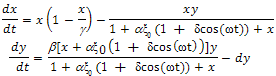 | (3) |
In this paper, we first compare the biological control path of the system (3) in presence of both low and high quality of additional food to predators by varying the strength of fluctuations parameter δ in section 2. We have also analysed the dynamics of this model through bifurcation analysis with respect to strength of fluctuations parameter δ and angular frequency ω for low as well as high quality of additional food respectively in section 3. Finally conclusion is given in section 4.
2. Predator-Prey Control Path Due to Strength of Environmental Fluctuations
In this section, we have studied some important observations of the dynamics of system (3) through numerical simulations. We have analysed the path of controllability of the system (3) with additional food to predator. According to Srinivasu et al[6], the additional food is of high quality if α < β/d and it is of low quality if α > β/d. Here we have analysed the biological controllability for both cases of α. We have considered the ecosystem parameters as γ = 6.0, β = 0.3, d = 0.2, ω = 0.1 and different values of δ in the range 0 ≤ δ ≤ 1.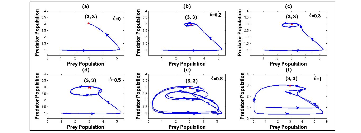 | Figure 1. Biological control path of predator-prey system (3) for different values of parameter δ taking low quality of additional food α = 2, ξ0 = 1 for predator. |
We first take low quality of additional food and choose α = 2, ξ0 = 1 for predator. We fix the target level (x∗, y∗) to be (3, 3). Taking without any fluctuation δ = 0, from figure 1(a), we observe that it is possible to reach the target state (3, 3) starting from the initial point (1, 1). This indicates that it is possible to reach target state exactly for the system (3). Taking the strength of fluctuation δ = 0.2, the figure 1(b) shows that the system (3) cannot reach the target state exactly, but it is possible to reach small neighbourhood of the equilibrium point(3, 3) initiating the path at(1, 1) through limit cycle. From figure 1(c), figure 1(d), figure 1(e) and figure 1(f), we observe that it is not possible to reach the target state. But we also observe that the periodicity of the control path changes significantly depending on the value of δ. That is the dynamics of the system (3) with seasonal variation is more complex than a system without seasonal effects.Next, we take high quality of additional food and we choose α = 1.1429, ξ0= 1.4. The control path of the system (3) with high quality of additional food starting from the point (1, 1) is shown in figure 2. In this case, we fix the target level to be (1, 3). From figure 2, we observe that it is impossible to reach the target state taking any value of δ ∈[0, 1]. It illustrate that the path of the system (3) tends to high periodic orbits around the target level (1, 3) for nonzero value of δ in (0, 1].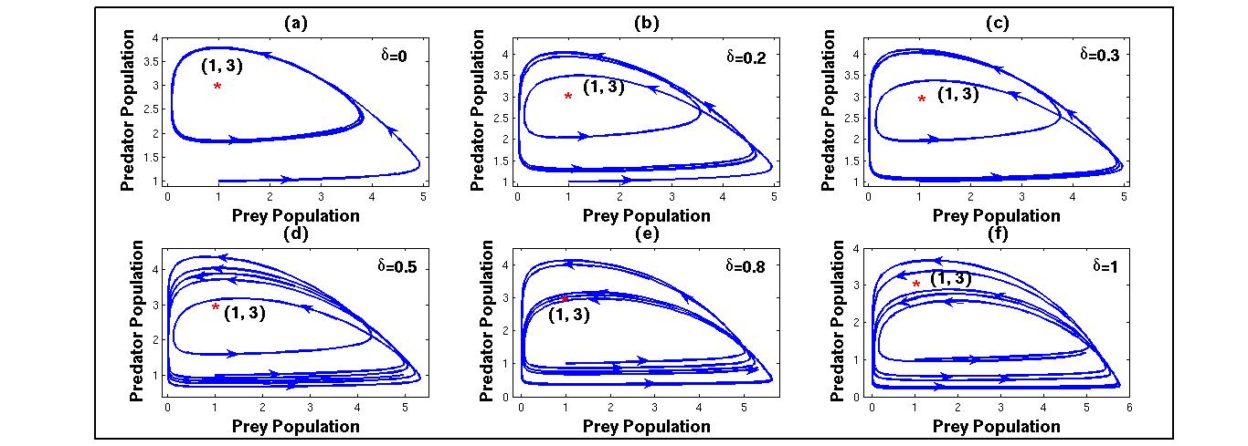 | Figure 2. Biological control path of predator-prey system (3) for different values of parameter δ taking high quality of additional food α = 1.1429, ξ0 = 1.4 for predator. |
Therefore, from the above discussions we can conclude that the system (2) with proper choice of additional foods to predator can reach a target level. On the other hand for the system (3) we cannot reach exactly the target level but oscillates around the target. This means that if environmental fluctuation is taken into account the supply of additional food is not sufficient to control the dynamics of a predator-prey system.
3. Bifurcation Analysis
Bifurcation analysis is an important tool to investigate the dynamics of a system. In this section, we investigate the biological controllability of the system (3) with additional food to predator assuming periodically varying quantity of additional food. We have done bifurcation analysis of the system (3) with the set of hypothetical ecosystem parameters, most of which are taken from Srinivasu et al.[6]. The parameter values are taken as γ = 6.0, β = 0.3, d = 0.2, which are remain unchanged throughout simulations. Here, we have done bifurcation analysis with respect to strength of fluctuation δ and angular frequency ω for both low and high quality of additional food to predator.We first fix low quality of additional food as α = 2, ξ0 = 1 and ω = 0.1. Figure 3 shows the bifurcation diagram with respect to strength of the fluctuation δ in the range 0 ≤ δ ≤ 1. The resulting bifurcation diagrams figure 3(a) and figure 3(b) shows that the system (3) has a dynamics including limit cycles, period-2 orbits. Next, we allow the high quality of additional food α = 1.1429, ξ0= 1.4 for predator. From figure 3(c) and figure 3(d), we can conclude that the dynamics of the system (3) shows limit cycle and high periodic orbits. Figure 3 depicts that the prey population have high extinction risk.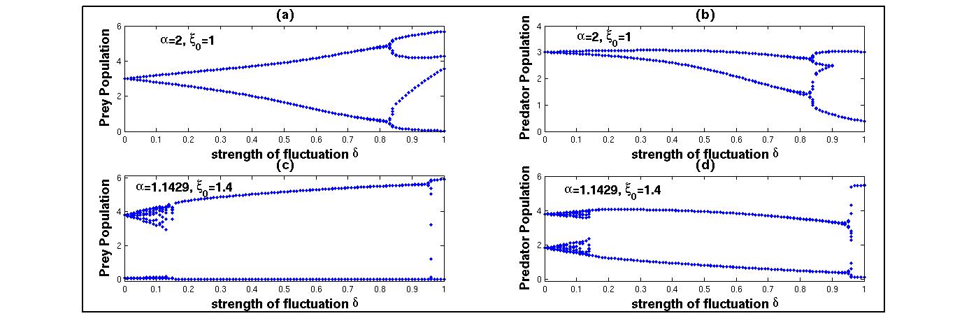 | Figure 3. Bifurcation analysis of the model (3) with respect to strength of fluctuation δ with low and high quality of additional food to predator. |
Now, we have analysed the bifurcation diagram of the system (3) with respect to angular frequency ω for both low and high quality of additional food to predator taking δ = 0.1. Figure 4(a) and figure 4(b) are the bifurcation diagrams of the system (3) with respect to angular frequency ω taking α = 2, ξ0= 1. The figure 4(a), figure 4(b) shows that the system has limit cycle oscillations only. On the other hand, taking high quality of additional food α = 1.1429, ξ0 = 1.4, from figure 4(c) and figure 4(d), we can conclude that the system (3) have high periodic oscillations. The figure 4(c) and figure 4(d) also shows that prey population has extinction risk. Therefore, we observe that a two dimensional system produces more complex dynamics with seasonal variation than a constant environment. A two dimensional predator-prey system can be controlled with supply of additional food to predator. But a system with seasonal variation cannot be controlled with only additional food to predator. From bifurcation analysis we have observed that the system have high extinction risk.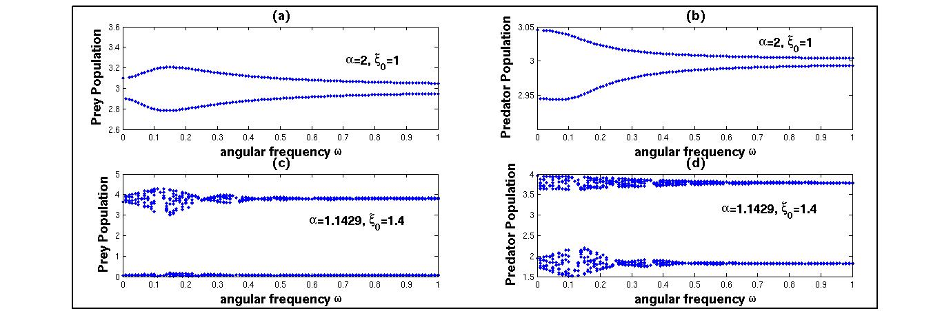 | Figure 4. Bifurcation analysis of the model (3) with respect to angular frequency ω with low and high quality of additional food to predator |
4. Conclusions
In this paper, we have investigated the dynamics of a predator-prey system with periodically varying quantity of additional food to predator. We have compared the control path of our model with the model having constant supply of additional food. We have done the bifurcation analysis of our model with respect to strength of fluctuation δ and angular frequency of oscillation ω separately for different set of parameters values. We have noticed that the modified predator-prey system with periodically varying quantity of additional food exhibits very interesting and complex dynamics. We can conclude that the system dynamics is highly affected by periodically varying quantity of additional. With constant supply of additional food, a system can reached the target point with suitable choice of additional food to predator, but a system with periodically varying quantity of additional food cannot reach the target point. It always oscillates around the target point for seasonal variation of quantity of additional food. In spite of the supply of additional food to predator, the bifurcation analysis shows that the system has high extinction risk due to environmental fluctuation. This means that if environmental fluctuation is taken into account the supply of additional food is not sufficient to control the dynamics of a predator-prey system. We suggest that the proper choice of additional food in biological conservation and pest control, the quality and quantity of additional food should be determined with the knowledge of angular frequency and strength of fluctuation of additional food.
References
| [1] | M.L.Rosenzweig, R.H. Macarthur, 1963, Graphical representation and stability conditions of predator-prey interactions, The American Naturalist, 97, 209-223 |
| [2] | S. Gakkhar, S.K. sahani, K. Negi, 2009, Effects of seasonal growth on delayed prey- predator model, Chaos, Solitons and Fractrals, 39, 230-239 |
| [3] | R.K. Upadhyay, S.R.K. Iyengar, 2005, Effect of seasonality on the dynamics of 2, 3 species prey-predator systems, Nonlinear Analysis:Real World Applications, 6 , 509-530 |
| [4] | Y. Do, H. Baek, Y Lim and D Lim, 2011, A three species food chain system with two types of functional responses. Abstract and Applied analysis, Article ID 934568, doi:10.1155/2011/934569 |
| [5] | K.P.Das, S. Chatterjee, J. Chattopadhyay, 2009, Disease in prey-population and body size of intermediate predator reduce the prevalence of chaos-conclusion drawn from Hasting-Powell model, Ecol. Comp., 6, 363-374 |
| [6] | P.D.N. Srinivasu, B.S.R.V. Prasad, M.Venkatesulu, 2007, Biological control through provision of additional food to predators:a theoretical study, Theor Popul Biol, 72, 111-120 |
| [7] | P.D.N. Srinivasu, B.S.R.V. Prasad, Time optimal control of an additional food provided predator-prey system with applications to pest management and biological conservation. Bull Math biol. 2009 |
| [8] | P.D.N. Srinivasu, B.S.R.V. Prasad, 2010, Role of quality of additional food to predators as a control in predator-prey system with relevance to pest management and biological conservation, Mathematical Biology 60, 591-613 |
| [9] | A. Gragnan, S. Rinaldi, 1995, A universal bifurcation diagram for seasonally perturbed predatorprey models, Bull. Math. Biol., 57, 701-712 |
| [10] | A.R. Ives, K. Gross, V.A.A. Jansen, 2000, Periodic mortality events in predator prey systems, Ecology, 81(12), 3330-3340 |
| [11] | S. Rinaldi, S. Muratori, Y. Kuznetsov, 1993, Multiple attractors, catastrophes and chaos in seasonally perturbed predator-prey communities, Bull. Math. Biol., 55, 15-35 |
| [12] | J.M.Cushing, 1977, Periodic time-dependent predator-prey systems, SIAM Journal on Applied Mathematics, 32, 82-95 |
| [13] | S. Gakkhar and R. K. Naji, 2003, Chaos in seasonally perturbed ratio-dependent prey- predator system, Chaos Solitons and Fractals, 15, 107-118 |
| [14] | G. C. W. Sabin and D. Summers, 1993, Chaos in a periodically forced predator-prey ecosystem model, Mathematical Biosciences, 113, 91-113 |
 Abstract
 Reference
 Full-Text PDF
 Full-Text HTML