1. Introduction

Repetitive construction projects require large amounts of resources that are used sequentially. Effective planning, scheduling, and controlling construction projects reduce construction time and reduce cost [1]. Different scheduling techniques have been proposed in the literature to satisfy such benefits, most of which are overshadowed by the Critical Path Method (CPM). Despite the wide application of CPM in construction management [2], it fails to schedule repetitive projects where the same basic unit is repeated several times [3,4,5,6,7]. The main shortcoming of CPM in repetitive project scheduling is its inability to ensure crew work continuity. Many other approaches have been developed to overcome the drawbacks of CPM techniques for scheduling repetitive construction projects. These include the 'Line of Balance (LOB)' method, 'and 'Linear scheduling method (LSM)'. [6,8]. These scheduling methods for repetitive construction projects focus on maximizing crew work continuity by enabling each crew to finish work in one unit of the project and move promptly to the next without work breaks. These methods aimed to finish the project at the earliest for a set of crew formations, but do not consider alternative resource crew formations. LSM can schedule projects and include recurring and non-recurring activities, typical and non- typical activities, serial and non-serial activities. Thus, in the current research, LSM is used due to its advantages.

The main objective of this paper is to develop a scheduling optimization model for recurring projects to identify the optimum solution that minimizes total project cost under a set of constraints considering different scenarios for incorporating Interruption, buffer time, and schedule acceleration. The previous models were considered one aspect only, such as Interruption or buffer time or acceleration when minimizing project duration or total cost. On the contrary, the proposed model considers these aspects in one model. Also, the current model is flexible for the user to choose some essential features such as: interruption percentage, over time factor used in acceleration, relative weights allocated to cost slope, and contractor's judgment.

The paper is organized as follows. The second section is devoted to reviewing literature concerned with scheduling problems. The third section explains the methodology adopted in the current research. Model development is described in the fourth section. A software program is prepared to automate the developed model in section 5. An example project is presented in section 6 to show how the model performs step by step. The results are discussed in section 7. Finally, conclusions are drawn, and recommendations for future work are highlighted in section 8.

2. Literature Review

Repetitive construction projects can be divided into two main groups: linear, such as highways, railroads, and pipelines, and nonlinear, such as high-rise buildings and multiple housing construction. Furthermore, repeated construction projects can be divided into two groups, as shown in fig. (1) Typical projects where activities have the same quantities, i.e., have the exact durations through all units, (2) Non-typical projects where activities have different quantities, i.e., have different durations through units [9].

In this class of projects, construction crews are often required to repeat the same work in various project units, moving from one unit to another. Due to this frequent crew movement, scheduling methods for repetitive construction projects focus on maximizing crew work continuity by enabling each crew to finish work in one unit of the project and move promptly to the next to minimize work interruptions. The application of work continuity improves the overall productivity of construction crews due to: (1) minimizing their idle time during their frequent movements on-site; and (2) maximizing their benefits from learning curve effects _ [10,11]. However, despite the advantages of crew work continuity, its strict application can lead to longer overall project duration, e.g. [3,12,13]. This led to a many research studies investigating the impact of crew work continuity on the planning and scheduling of repetitive construction projects, e.g. [5,14,8,15,11,16,17,18,19,20]. Due to the feature of repetition, the ideal use of resources is to maintain the continuity of work such that there is no idle time between units and crews and can flow through the project smoothly and without any work interruption or idleness [53].

Available planning and scheduling models that focused on minimizing the duration of repetitive construction projects can be grouped into two main categories: 1) models that provide strict compliance with crew work continuity [3]; and 2) models that allow interruptions to crew work continuity [5,11].

Several methods have been developed for determining the crew formations that minimize the project duration or cost. [3] proposed a dynamic programming model that considers crew formations as decision variables to minimize the project duration; but ignored work interruptions or decision-making costs. [5] developed a two-state variable, an N-stage dynamic model that considers a set of possible durations (for different available crew formations) and a set of interruption durations as decision variables to minimize the project duration. In another effort made by [9], they developed a dynamic programming model to reduce the project's overall cost by identifying the optimal crew. They considered typical and non-typical recurrent projects, resource constraints, and maintaining work continuity. Five years later [8] presented a dynamic programming model to reduce the project's overall cost by considering the work interruption and multiple crews for each activity simultaneously in repetitive units. [14] proposed a two-variable N-stage dynamic programming aimed at reducing the overall cost for scheduling non-serial activities. [15] presented a model based on dynamic programming formulation, designed to identify an optimum crew formation and interruption option for each activity in the project, leading to minimum project duration. [13] introduced an improved dynamic programming model to include a set of heuristic rules that reduce both the duration and the overall cost of the project. Another group of studies has adopted linear programming. [21] proposed a linear programming model to maximize the construction rate of the activities in a repetitive project. [4] utilized a linear programming formulation to minimize the direct project cost for given project duration. [22] presented a multi-objective linear programming model for scheduling optimization of repetitive projects, which considers cost elements regarding the project's Duration, the idle time of resources, and the delivery time of the project's units. [55] developed a linear optimization model for scheduling repetitive construction projects with varying quantities of work in repetitive units. The model provides new capabilities that enable planners to identify an optimal/near-optimal schedule that minimizes project total cost and number of times crew work is interrupted. [23] presented a multi-objective fuzzy linear programming model that considered the project's duration, the total cost, and the total time of interruptions simultaneously. [20] developed an advanced model programmed using the nonlinear programming method to achieve the minimum Duration of the project, considering a set of constraints, such as maintaining the continuity of work, resource constraints, work interruptions, and synchronization crews. [16] introduced a repetitive scheduling model to minimize total project cost integrating CPM and LOB considering only linear (horizontal) repetitive projects. [18] developed a multi-objective genetic algorithm model for optimizing resource utilization in redundant infrastructure linear projects. [17] presented a model to assign resources to activities in linear repetitive projects optimally. The model trades off between work interruption and project duration using genetic algorithms. In conclusion, many formulations for repetitive projects have been developed focusing on minimizing project cost or minimizing project duration. [54] developed integrated model of CPM and LOB with fuzzy time data for scheduling repetitive projects is presented. The developed model provides a new technique to schedule repetitive projects with fuzzy time data in an easy non-graphical manner. [56] developed a time-cost optimization model to schedule repetitive projects while considering limited resource availability.

Buffer building is another domain for recurrent projects. Buffer is an essential element of the project's recurring schedules because resources are already on-site, and therefore, any delay in activity has a more significant cost impact than traditional projects. Thus, the balance line is used for buffers to protect continuity and force the minimum distance or time between sequent activities and avoid overlapping crew and site congestion during implementation. Recent efforts presented methodological buffer sizing techniques that can be classified into two main classes. The first class is for sizing buffers techniques based on historical data in activities durations' statistical distributions. Such techniques build buffers based on factors such as the ratio of a duration's standard deviation to the mean, the coefficient of variation, or the difference between the 90 per cent probability completion duration and the mean duration [25,26,27,28]. The best methods are R.D. medium safety, RESM and, BLUE, which provide statistically appropriate buffer ranges closer to the other methods provided in the literature review [29]. The second class comprises sizing buffers techniques given specific factors that increase the impact of delays on the schedule, such as the activities’ location in schedule, the number of precedence relations of each activity, activities durations, resource tightness, degree of fuzziness, or factors reflecting uncertainty in the law, economy, social and technological environments surrounding the project [30,31,32, 33,34,35].

In the construction industry, contractors may need to accelerate projects to recover from delays during work, benefit from the contractual bonus, avoid penalties, and/ or avoid undesirable weather conditions and site. On the other hand, owners may need to accelerate projects to take advantage of market opportunities and / or meet financial requirements and commercial requirements. The acceleration of the schedule addresses finding an accurate balance between the increased in direct cost, the allocation of additional resources, and the indirect cost reduction, because of the short duration of the project [36].

Previous techniques used to speed up project schedules at both strategic and tactical levels can be divided into six main groups. These are (1) heuristic procedures [37, 38, 39]; (2) mathematical programming [40, 41]; (3) simulation [42]; (4) genetic algorithms [44]; (5) integration of simulation with genetic algorithms [45,46,47], and (6) genetic algorithms and fuzzy set theory [48,49].

However, all these techniques address traditional (non-recurrent) projects. On the other hand, the acceleration of recurrent construction projects is faced with additional challenges: (1) identifying activities for acceleration, which is not as easy as in regular, non-recurrent projects. (2) Compliance with the crew work continuity constraint. In recurrent projects, there are no identical means to define the series of critical activities or parts of activities that control the project's overall Duration and can be used to speed up the schedules [50,51]. In previous studies, two algorithms were found to identify accelerated activities in recurring project schedules. These algorithms use the relative alignment of successive activities to identify activities that need to be accelerated in recurring projects [51,52]. Less aligned activities are activities that progress at a lower rate than their successor. Acceleration of such activities would lead to a shortening of their Duration, advance the start date of subsequent activities, and shorten the project's overall duration. If a higher activity is accelerated than its direct successor, the direct cost of the project will increase without any reduction in the overall duration of the project. On the other hand, activities with a higher rate than their predecessor and a lower rate of a successor have been identified as converging activities. By relaxing a converging activity's rate or introducing an intentional break, it can start earlier, and its successor can start earlier, as shown in fig. 1 [51]. Relaxing in an activity may be less expensive because it leads to fewer resources, but it may cost more. For example, relaxation in an activity may increase the rental period of the equipment and an increase in person-hours.

There are common acceleration strategies, which project managers often use when accelerating repetitive projects [51]. These strategies include: (1) working overtime; (2) working double shifts; (3) working weekends or (4) employing more productive crews. Additional costs accompany each of the acceleration strategies mentioned above. Examples of these additional costs are increased direct costs as labor wages and equipment running costs, and loss of productivity due to congestion in increased crew size [50]. On the other hand, as projects' total duration decrease, indirect costs also decrease.

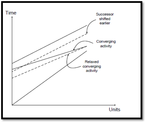Figure 1. Acceleration by Relaxing Converging Activities [52]

3. Research Methodology

A standard methodology is adopted in the current research. Before developing the proposed model, it's characteristics are presented. The proposed model considers many constraints that should fit the characteristics of scheduling repetitive construction projects. These constraints are activities logical relationships, duration constraints, interruption constraints, buffer constraints and acceleration constraints to identify the optimum solution that minimizes total project cost. The buffer sizes will be inserted between successive activities. The acceleration addresses finding the balance between the increase in direct cost, due to assigning additional resources and the decrease in indirect cost, due to shortening project duration. Consequently, the main challenge is to identify the acceleration strategy that would require the least amount of additional cost. The final model is an optimization model that generates several trade-off solutions between the duration of the project and the total project cost.

The scheduling technique used to represent the product schedule is LSM. Four scenarios are adopted to study the effect of allowing Interruption, project buffers, and schedule acceleration on the traditional time/cost trade-off. These scenarios are as follows:

1. The first scenario is a traditional time/ cost trade- off, which does not allow Interruption, buffer constraints, or schedule acceleration.

2. The second scenario allows Interruption.

3. The third scenario considers project buffers only.

4. The fourth scenario considers schedule acceleration only.

Software is prepared to automate the developed model because the scenario of schedule acceleration requires software. Also, all scenarios for large- size projects could not be applied without software. The software is prepared using a c # programming language. An example with a small number of activities is presented to show how the model performs. The results are presented and discussed The conclusion and further extensions are then provided.

4. Model Development

The developed model consists of scheduling and optimization modules. The scheduling module develops practical schedules for repetitive construction projects. At the same time, optimization modules look for optimized solutions to achieve specific functions.

After performing these basic calculations for all possible crew formations, the objective function in Equation 1.

(1)

Where: is the total cost of the project; is the direct cost of activity i; is the total penalty in interruption cost for activity i; is the total indirect cost of the project; is the acceleration cost of unit the is the total number of accelerated units.

Scheduling Module

The principal objective of this module is to develop a project activities schedule in all the repetitive units. This module incorporates two main components scheduling component responsible for the optimal scheduling process and the buffer component responsible for sizing and inserting time buffers.

Scheduling component

This component is designed to deal with typical and non-typical repetitive activities. It computes the scheduled start and finish times for any activity in any repetitive unit the total project duration the total number of crew interruption days and the total project cost . This computation of scheduling is carried out in two stages, as follows.

a) First stage

At this stage, the model creates a schedule that respects the logical job constraints, maintains continuity of work and crew availability. For an activity in the unit using the quantity of work and the daily production rate of the selected crew option, the duration is calculated by Eq. 2:

(2)

At this stage, the early start for crew formation is identified due to crew availability and job logic constraints. The early start time can be calculated due to crew availability using the following equations:

For the first unit, the crew is assigned to

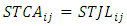(3)

Where: is the start time due to crew availability of activity at unit ; is the start time due to job logic of activity at unit .

For remaining units

(4)

Where: is the early finish time of activity i for crew

A special case appears when one crew is assigned to repetitive activities as in Eq. (5):

(5)

The early start time can be calculated due to job logic and precedence relationships between activity and its precedence. These relationships may be either finish to start, finish to finish, start to start or start to finish with or without lag time. This is achieved by restricting the start time according to the job logic so that each activity is greater than or equal to the maximum finish time of the schedule of previous activities plus lag time. For start activities, the start time due to job logic is zero in all units as specified by Eq. (6). When calculating the start time according to the job logic of other activities, the lag time must be added to the scheduled finish time of the previous activity as specified by Eq. (7).

(6)

(7)

Where: is the start time due to job logic of activity at unit is the number of predecessors; is the finish time of the previous activity of predecessor .

The start time of successor activity due to crew availability is then compared with the start time according to job logic, and the latest value of the two is identified as the early start time of the unit as given in Eq. (8)

(8)

Where: is the early start time of activity at unit .

When the early start time is calculated, the early finish time for any activity is given by Eq. (9)

(9)

Where: is the early finish time of activity at unit .

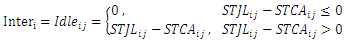
After this stage, as soon as possible, all activities are scheduled. Then, crews are assigned to the units, and the early start time and early finish time are calculated. However, there is no warranty to maintain work continuity constraints for all crews. Therefore, the second stage is responsible for checking and updating work continuity constraints for all crews.

b) Second stage

When the starting time due to job logic is later than the start time due to the availability of the crew, the crew then sits idle until the work is completed from the previous activities. The time when the crew is idle is equal to the difference between the previous two times. On the other hand, if the start time according to the job logic earlier than the start time according to the availability of the crew, it means that the activity starts immediately because the crew will be available to work immediately, in this case, there is no idle time for the activity. Eq. (10) represents these cases

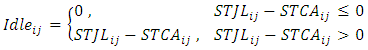(10)

Where: is the idle time of activity i at unit j.

The second stage is designed to achieve compliance with the work continuity constraints by resetting the scheduling established in the first stage to ensure that it satisfies the continuity of the crew. This is achieved by shifting the schedule of activities developed for the first stage, if necessary, to prevent the idle time of any crew. To remove idle time, the start time of activity i in- unit j must be changed with a value equals to the sum of all idle times for the subsequent units assigned to the same crew in an activity. The shift is defined as the aggregation of all unforced idle times for subsequent units assigned to the same crew in an activity that can be delayed for each unit without delay the total finish time of the activity and can be expressed as described in Eq. (11)

(11)

Where: is the shift of activity at unit for crew n; J is the total number of units; and is the collection of all idle time of activity at units from to for crew

Thus, the specified shift for each unit is used to shift the scheduled start and finish times generated at the first stage given by Eqs. (12) and (13)

(12)

(13)

Where: is the shift of scheduled start and finish times comply with the crew work continuity constraints.

The schedule developed at this phase complies with crew work continuity constraints by shifting the start and finish times of some units. However, this may delay subsequent activities and extend the overall project duration, increasing the indirect cost. On the other hand, work interruptions sometimes reduce the Duration of the project and indirect costs and increase the direct cost. Therefore, a real trade-off between these two extremes should be made.

Interruption constraints

Interruption can be used to shift the activity schedule into the specified units to start and end on a date earlier than the date specified in the second stage, resulting in a reduction in the project's duration. Therefore, Interruption of any activity is calculated as shown in Eq. (14):

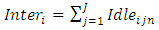(14)

This Interruption may result in additional costs due to resource mobilization or productivity losses due to a disruption of work continuity. The penalty interruption cost () for any activity (i) is applied to the total interruption time for each activity. This means that each activity has its own penalty interruption cost and is calculated by multiplying the time of Interruption for activity (i) by the penalty interruption cost per time unit of activity i using Eq. (15).

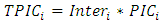(15)

Where: is the total penalty in interruption cost for activity i; is total Interruption of activity i; is penalty interruption cost per time unit of activity i.

Where:

(16)

According to the agreement, this ratio will be selected, the study of site conditions, project size, and the number of crews. In the current research, this ratio is assumed to be 60%.

Buffer component

Buffer sizing

The buffer size estimation methods were presented in detail in the literature review. In the current research, the R.D. method presented by Shou and Yeo, 2000 will be used to calculate buffer size. In his work, (Shou and Yeo, 2000) gave that if the most likely completion (), then the optimistic completion time (a) equals 0.75, and the pessimistic completion time (b) equals 2.

First, the planner calculates the R.D. value by using Eq. (17), then he specifies the desired level of safety to identify the buffer percentage (see Table 1). Finally, the planner determines the buffer for each activity by multiplying the buffer percentage through each activity's mean duration.

Table 1. Buffer size of different activities and safety levels [25]

(17)

Where: is the relative dispersion; is the standard deviation of activity; is the mean duration of activity

x The mean duration of activity can be calculated in each unit using Eq. (18).

(18)

x The standard deviation of activity can be calculated in each unit using Eq. (19).

(19)

Buffer insertion

After calculating the buffer for each unit, it should be inserted in the scheduling. Thus, to allow inserting the buffer, the activities must be shifted again, so there are two shifts for each activity: the first shift to maintain continuity of resources and the second shift to insert the buffers. The second shift is equal to summating the previous unit's buffers until the least Duration between two successive activities. Then the final scheduled start and finish times after calculating crew work continuity and intermediate buffers are calculated by applying Eqs. (20) and (21). Finally, the total cost of the project is recalculated according to the total new project duration.

(20)

(21)

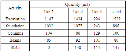
Where: is the required shift to ensure crew work continuity; is the required shift to accommodate inserted buffers.

Acceleration constraints

The acceleration step is optimized using a genetic algorithm, which is an evolutionary-based optimization technique. An optimization process for interruption removal scenarios is required because the interruption removal step is unpredictable and can only be solved using an exhaustive search. An exhaustive search in our case will be very inefficient in searching for a wide range of values, so an evolutionary-based optimization such as a genetic algorithm is used for selecting the acceleration activities.

• The additional cost of acceleration

To determine the additional cost of acceleration, the strategy used for acceleration is defined as overtime, and the cost of over time for each activity unit is calculated using the following Eq. (22).

(22)

In this research, a value of 2.5 is used for overtime factors as adopted [52]. Then the cost of accelerating each activity is calculated to shorten the project duration by one day (one- day affect cost).

• Schedule of Acceleration

In the activities appointed for acceleration, each unit has two separate priority rankings; one is the priority of the cost slope and the other is the priority of the contractor's judgment Both are combined to produce a joint priority utilized in the queue of activities for acceleration. Relative weights are utilized to determine the relative importance of two classification criteria. The user assigns the prioritization process according to his specific needs by using these relative weights. Increasing the weight of the cost slope will make the joint priority produced for activity more relying on the priority of cost slope and vice versa. For example, if the user desires to create an equal acceleration plan based on the cost slope and contractor judgment, both weights will be assigned 0.5. On the other hand, if he desires his decision to be more dependent on the cost slope than the contractor's judgment, he will allocate a weight of 0.6 for the cost slope and 0.4 for the contractor's judgment. Weight 1.0 for the cost slope and 0.0 for the contractor's judgment would create a less cost acceleration plan. When the user experiences this method, he will put weight values appropriate to his preferred needs. However, the joint priority is calculated according to Eq. (23).

(23)

Where: is of any segment (element).

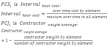
is the relative weight allocated to the cost slope is the relative weight allocated to the contractor's judgment

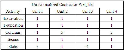
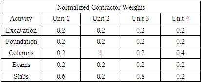
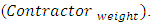The actual acceleration begins after the calculation of joint priorities. First, it is implemented by gradually allocating acceleration resources to the unit with the lowest joint priority. Then, acceleration resources are inserted, considering each one provides the maximum resource. Accordingly, the Duration of the unit is reduced to the new accelerated Duration, and the remainder of the schedule and costs of the project are recalculated. This method applies during the project implementation stage, i.e., after signing the contract and the beginning of construction on the site.

After each unit is accelerated, the program recalculates the schedule, and the new total cost and duration of the project are signed. This process is repeated in a repetitive method until the target duration or the target cost is accomplished.

Steps of acceleration:

1. The Gantt chart is drawn with the start and finish times for each activity in each unit.

2. The cost of over time for each activity unit is then calculated using Eq. (3.22).

3. The Gantt chart is then divided into parts, representing a segment with the exact cost.

4. Calculate over time cost for each segment (element).

5. There are two cases of acceleration in this thesis:

x First Strategy (cost slope only): in this scenario the contractor's judgment is given a weight equal to 1 for each unit in each activity. Then, a normalization of each value is done by dividing each value by the maximum one.

x Second Strategy (cost slope and contractor judgment): in this scenario, the contractor's judgment is given weights based on his experience. Then a normalization of each contractor's judgment is done by dividing each value by the maximum one.

6. The combined intervals weight for each element is then assigned based on the cost slope () and contractor's judgment () using Eq. (3.23).

7. Then accelerate segments with the lowest combined intervals weight so that the segment is not compressed more than two-thirds of the time.

5. Developed Software

C # programming language is selected due to its powerful programmability features and ease of use. The program provides the planner with simple data entry of the activities; name, sequence, logic (precedence relations), and durations. In addition, the C # programming language allows dynamically changing the schedule according to the inputs provided to the model. Implementation and optimizing the scheduling of recurring project activities are performed as follows:

1. Put input primary schedule data and then Perform schedule optimization to obtain Optimum crew formation, leading to the least cost.

2. Create a model for sizing and inserting time buffers to protect the schedule against expected delays.

3. Allow Interruption of work because it sometimes reduces the Duration of the project and indirect costs.

4. Develop an automated acceleration model optimized for recurring projects.

6. Model Implementation

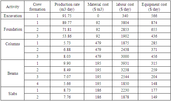
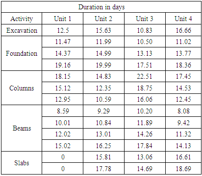
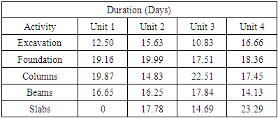
A concrete bridge example is presented to show the performance of the proposed optimization model and demonstrate its capabilities. This example was initially introduced by [3] and later analyzed by [5,9]. The project consists of four similar units, and each one includes the following repetitive activities: excavation, foundations, columns, beams, and slabs. Each repetitive activity is performed by a crew that progresses from the first to the fourth section sequentially. The job logic (i.e., relationships) among succeeding activities is finished to start with no lag time. Available crew formations associated with each activity with different costs and productivity are listed in (Table 2) [3]. Table (3) shows the quantities of activities in for the original example. Four scenarios will be adopted to identify the optimum solution that minimizes the total project cost.

Table 2. Crews Production rate and direct cost for the example project [3]

Table 3. Quantities of activities for the example project [3]

The available number of different activity crews can provide 72 different crew formations for the project. Therefore, the solution begins by listing all possible crew formations, calculating their respective durations and costs.

The first scenario does not consider both schedule acceleration and buffer constraints and does not allow Interruption.

Duration and cost for Excavation activity

Applying Eq. (2) to calculate durations of different units using tables (2) and (3)

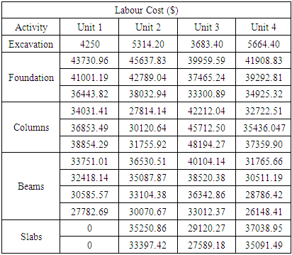
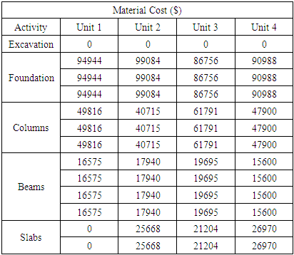
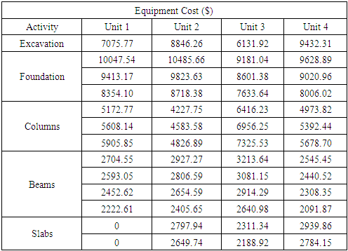
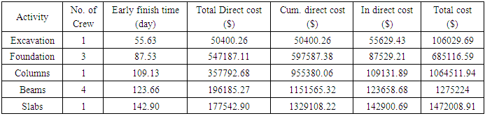
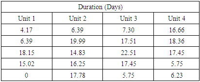
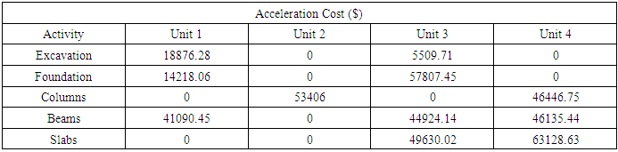
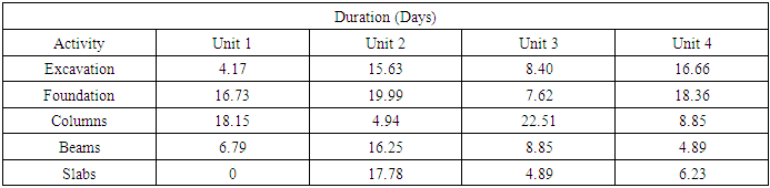
Duration for unit 1 = =12.5 days

The same equation is used for the rest of the activities in all units to calculate their duration, as shown in table (4).

Cost calculation for Excavation activity

x L Labor cost = Duration * Labour cost ($/day)

Labour cost for unit 1 = 12.5 (see table 4) * 340 (see table 2) = $ 4250

The same equation is used for the rest of the activities in all units, as shown in table (5).

x Material cost = Quantity (m3) (see table 3) * Material cost ($/m3) (see table 2)

Material quantity for unit 1 = (0) (see table 3) * (0) (see table 2) = 0

The same equation is used for the rest of the activities in all units, as shown in table (6).

x Equipment cost = Duration (see table 4) * Equipment cost (see table 2) ($/day)

Equipment cost for unit 1 = 12.5*566 = $ 7075

The same equation is used for the rest of the activities in all units, as shown in table (7).

Several attempts have been made, and it is found that the optimum crew formation selection consists of one crew for excavation (E1), three crews for foundation(F3), one crew for column (C1), four crews for beams(B4), and two crews for slabs (S2). The operation determined the optimum crew formation to be E1 F3 C1 B4 S2 resulting in the lowest total cost of $ 1472008.91and a corresponding 142.9 days. Table (8) shows the Calculation of the scheduling module. Table (9) shows the calculation of total cost. It must be noted that the indirect cost is calculated by multiplying early finish time by indirect cost per day ($1000).

Table 4. Calculation of Duration for all activities for different units

Table 5. Calculation of Labour cost for all activities for different units

Table 6. Calculation of Material cost for all activities for different units

Table 7. Calculation of equipment cost

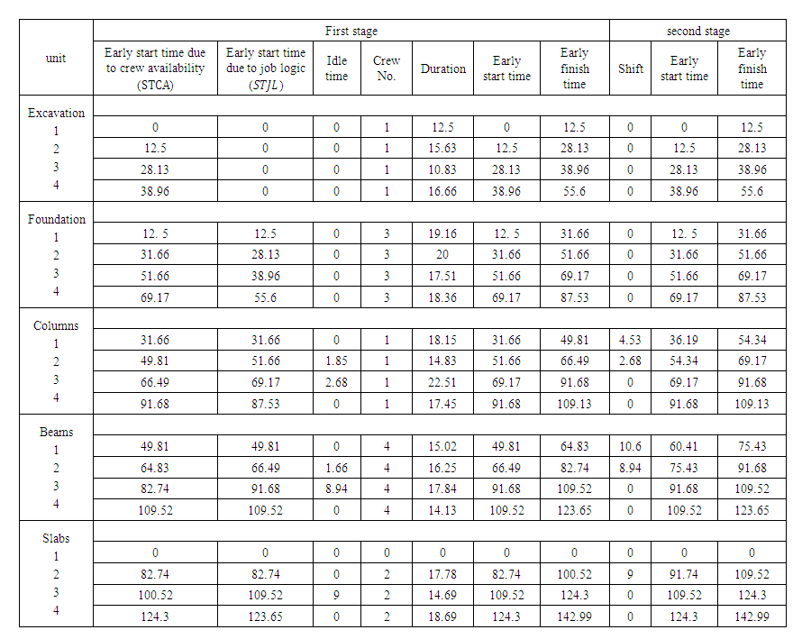Table 8. Calculation of scheduling module

Table 9. The total cost of optimum crew formation

The second scenario: allows Interruption

Calculate penalty interruption cost per time unit of activity

(16)

For Excavation activity

If a percentage of 60% is applied, for example, as an interruption percentage and using labor cost and equipment cost is given in table (2).

= 60% (340 + 566) *91.75 = $ 49875.3

Calculate total penalty in interruption cost for activity i

(15)

(10)

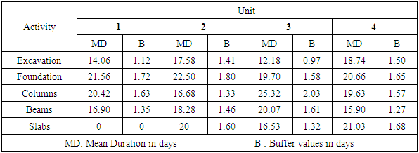
For unit 1= 0 * 49875.3 = 0

The same previous equations are used for the rest of the activities.

This scenario results are the lowest total cost of $ 1473912.34 and a corresponding duration of 142.90 days.

The third scenario considers project buffers only

Calculate the mean duration of activity in each unit

(18)

For Excavation activity

Using durations of different units (see Table 4) and substituting about by 12.5 in Eq. (18), is calculated for each unit. As previously mentioned, a = 0.75, b = 2

for unit 1 = =14.06 days

Calculate the standard deviation of activity in each unit

(19)

for unit 1 = 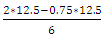= 2.60 days

Calculate the relative dispersion of activity in each unit

For unit 1 = = 0.185

The planner will use the desired level of safety and activity category and specifies the required buffer percentage for each activity from the table (1)

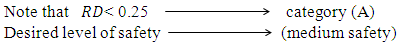Then buffer percentage = 8% =0.08 for all units

Then buffer is generated by multiplying the buffer percentage by the mean duration for each activity.

Buffer of unit 1 = 0.08 * 14.06 = 1.12days

The same steps are adopted for all units in all activities to calculate their buffer.

Table (10) summarizes the calculation for the mean duration of activities and buffer calculation of activities.

Table 10. Summary of Mean Duration and Buffer of activities

The second shift is equal to the summation of the previous unit's buffers until the least Duration between two successive activities, as shown in table (11). The least duration between two successive activities is equal to the bigger of the first shift, where the first shift is defined as the aggregation of all idle times for subsequent units assigned to the same crew in an activity as per Equation (11). To calculate the second shift of the Columns activity, the least Duration was found at the first unit (4.53) as highlighted in Table (8), then the second shift is equal to the summation of the previous unit's buffers until the least Duration between two successive activities (1.72). Then the final scheduled start and finish times after calculating crew work continuity and intermediate buffers are calculated by applying Eqs. (18) and (19). Table (12) shows the new duration of activities.

Table 11. Calculation of second shift

Table 12. New Duration of activities

The results of this scenario are the lowest total cost of $1476613.30 and a corresponding duration of 147.51 days.

The fourth scenario considers schedule acceleration only.

§ The Gantt chart for the initial schedule in scenario 1(first stage) is drawn with each activity's start and end times in each unit.

The overtime cost for each activity unit in each activity is then calculated using Eq. (22).

(22)

For Excavation activity

By substituting in Eq. (22) and applying an overtime factor equal to 2.5.

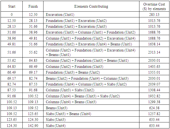
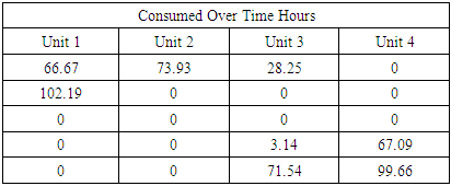
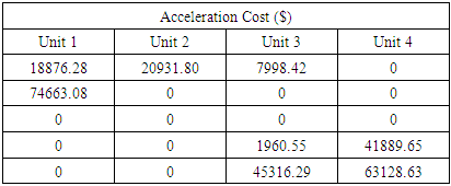
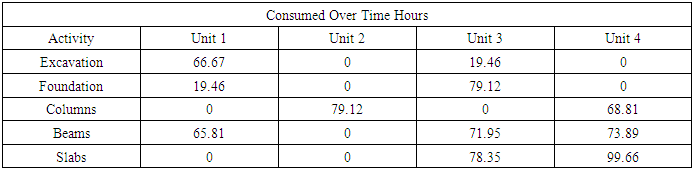
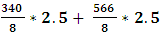Over time cost in unit 1 = = 283.13 $/hr

The overtime cost for the rest of all units in all activities is calculated using the same equation. Thus, the overtime cost for any unit of foundation, columns, beams, and slabs activities is $ 730.63, $ 675, $ 624.38, and $ 633.44, respectively.

§ Then the Gantt chart is divided into parts, representing a segment with the exact cost. We notice that we have 19 segments, as shown in Fig. 2. Table (13) shows each segment's start and finish time, elements contributing to overtime cost, and the corresponding overtime cost.

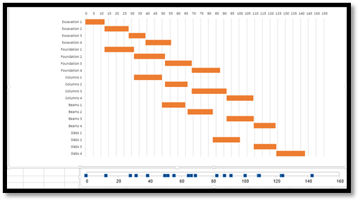Figure 2. Gantt chart

Table 13. Over time cost for different elements contributing

The first option (scenario 4a: cost slope only)

This option aims to create a least- cost acceleration plan without accounting for the contractor's judgment. In this option, the contractor's judgment is given a weight equal to 1 for each unit in each activity, as shown in table (14). Then, a normalization of each value is done by dividing each value by the maximum one. Since the un normalized contractor's judgment weights are 1 for all units in all activities, the normalized contractor's judgment weights are 1 for all activities.

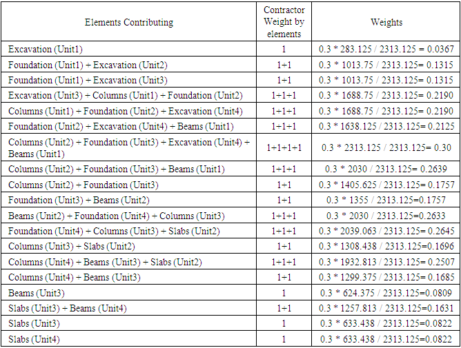
§ A combined interval weight for each element contributing is then assigned based on the cost slope () and contractor's judgment () using Eq. (23). Weights for cost slope (0.3) and contractor's judgment (0.7). Table (15): shows the calculation of combined intervals weight.

Table 14. Un-normalized contractor's judgment weights

Table 15. Calculation of combined intervals weight

Units with the lowest combined intervals weight are then accelerated.

Checking table 15 shows that unit 1 in excavation activity possesses the lowest combined intervals weight. Unit 1 in excavation activity has a duration of 12.5 days, i.e., 100 hours. It is found that this unit has compressed to one – thirds of the time. In other words, the compressed time for acceleration is 66.67 hours. Applying the overtime cost per hour, which was previously calculated as 283.13 $ /hr. This unit in this activity leads to an additional cost of accelerating of an additional cost of $ 18876. 28. Table (16) Shows consumed over time hours. Table (17) shows acceleration cost. Table (18) shows the new duration.

Table 16. Consumed Over Time Hours

Table 17. Acceleration Cost

Table 18. New Duration after applying acceleration

This scenario results show that the lowest total cost is $ 1704209.27, from which the acceleration cost is $ 274769.54 and the corresponding Duration is 100.33 days.

The second option (scenario 4b: cost slope and contractor judgment)

The second option aims to create a least- cost acceleration plan considering the contractor's judgment of the additional queuing criterion. In this option, the contractor's judgment is given weights as shown in table (19). Then a normalization of each contractor's judgment is done by dividing each value by the maximum one as shown in table (20).

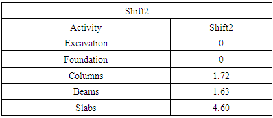
§ A combined interval weight for each element contributing is then assigned based on the cost slope () and contractor's judgment () using Eq. (21). Weights for cost slope (0.3) and contractor's judgment (0.7). For example, Table (25) shows the calculation of combined intervals weight.

§ Units with the lowest combined intervals weight are then accelerated, which are slabs (unit 3) with combined intervals of 0.2222 as from table 21.

Table 19. Contractor's judgment weights

Table 20. Normalized contractor's judgment weights

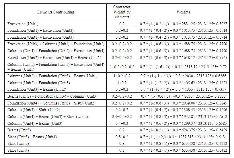Table 21. Calculation of combined intervals weight

Unit 3 in slab activity has a duration of 14.69 days, i.e., 117.52 hours. It is found that this unit has compressed by 78.35 hours. Applying the overtime cost per hour, which was previously calculated as 633.44 $ /hr. This unit in this activity leads to an additional cost of acceleration of $ 49630. 02. Table (22) Shows consumed over time Hours, Table (23) acceleration cost, whereas Table (24) new duration.

Table 22. Consumed Over Time Hours

Table 23. Acceleration Cost

Table 24. New duration after applying acceleration

This scenario shows that the lowest total cost is $1870211.79, from which acceleration is $ 441170.74 and the corresponding Duration is 99.93 days.

7. Results

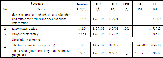
Table (25) shows the results. The project durations are 142.9, 142.9, 147.5, 100, and 99.9 days for scenarios 1, 2, 3, 4a and 4b, respectively. Whereas, the project total costs corresponding to these scenarios are $ 1472009, $ 1473912, $ 1476613, $ 1704210 and $ 1870212, respectively.

Table 25. Summarization of the results of the adopted four scenarios

8. Discussion

Table (25) summarizes the results of the adopted four scenarios. Comparing the case allowing Interruption (scenario 2) with the traditional case, which does not allow interruption, buffer, and acceleration (scenario 1), reveals that for the same duration, a slight increase in total cost equals 0.13% occurs. Considering buffer only and comparing this case (scenario 3) with (scenario 1) indicates an increase in project duration equals 1.03%, whereas the total cost increases by 1%. Applying acceleration to the initial schedule (scenario 1) considering cost slope (scenario 4a) reduces project duration by 30% and increases total cost by approximately 15.8%. These percentages are 30% and 27.1% when considering contractor judgment in addition to cost slope (scenario 4b).

9. Conclusions

Reviewing the literature revealed that: 1) the general lack of tools and techniques designed for optimal scheduling of recurring construction projects, 2) the difficulty of using tools and techniques designed for traditional projects to manage recurring projects, 3) the lack of a capable comprehensive buffering approach to address the primary sources without relying on relevant historical data and, 4) the inability of current technologies to account for acceleration costs and other influencing factors. To overcome these limitations, an optimization scheduling model considers many constraints that should fit the characteristics of scheduling repetitive construction projects has been developed. These constraints are activities logical relationships, duration constraints, Interruption constraints, buffer constraints and acceleration to identify the optimum solution that minimizes total project cost. The developed model studied the effect of allowing Interruption, project buffers, and schedule acceleration on the traditional time / cost trade-off through four scenarios.

Some contributions of the developed, optimized model have been made and listed below:

• Scheduling and interruption module capable of optimizing schedules for the least total project cost.

• Scheduling and buffering module of optimizing schedules for the least total project cost.

• A buffering approach has been developed that provides a structured tool for building buffers to protect the project schedule from expected delays.

• A schedule acceleration module comprises a unit-based acceleration algorithm capable of finding least- cost acceleration plans through accelerating units instead of activities.

• Queuing criteria for schedule acceleration allow considering cost slope and contractor's judgment while prioritizing units for acceleration.

Despite the capabilities and benefits of the proposed model, it has some limitations. The primary limitation is that the schedule optimization model is a single objective model that addresses either cost or duration, but not both.

The Proposed model can be implemented to different construction repetitive activities projects effectively. However, the presented model in this research could be improved considering the following points:

• Combine non-recurring and repetitive activities into one scheduling and optimization model.

• Experiment with different evolutionary algorithm optimization techniques that discover the solution space more effectively and efficiently (Particle Swarm Optimization, Ant Colony and Shuffled Frog Leaping algorithms).