Ahmed Senouci1, Ricardo M. Leon1, Neil Eldin2
1Department of Construction Management, University of Houston, Houston, USA
2College of Technology, University of Houston, Houston, USA
Correspondence to: Ahmed Senouci, Department of Construction Management, University of Houston, Houston, USA.
| Email: |  |
Copyright © 2019 The Author(s). Published by Scientific & Academic Publishing.
This work is licensed under the Creative Commons Attribution International License (CC BY).
http://creativecommons.org/licenses/by/4.0/

Abstract
Earned Value Management EVM has become a viable tool to measure project performance over the last four decades. Its ability to effectively monitor projects budget is widely accepted in the industry and academia. However, this tool has limitations that deserve attention. For example, its Schedule Performance Index SPI has a complete reliance on cost. This complete reliance on cost coupled with overlooking the fundamentals of (CPM) and its duration calculated approach to project performance may lead to misleading information. This paper examines instances where project SPI and CPM duration provide conflicting schedule indicators that could result in wrong decision-making. The SPI may sometime indicate that a project is ahead of schedule, while the CPM calculations show that the project is behind schedule. A simulation was created to generate project schedule scenarios in which SPI and CPM calculations provided conflicting schedule information. These scenarios were further examined to determine the cause of conflict between the two indicators.
Keywords:
Critical Path Method, Earned Value method, Schedule Performance Index, Cost Performance Index, Schedule Simulation, Project Schedules
Cite this paper: Ahmed Senouci, Ricardo M. Leon, Neil Eldin, Schedule Performance Index Effectiveness in Assessing Project Schedule Performance, International Journal of Construction Engineering and Management , Vol. 8 No. 2, 2019, pp. 46-55. doi: 10.5923/j.ijcem.20190802.02.
1. Introduction
Earned Value Management EVM is a technique for measuring project performance. It aims at measuring and evaluating the actual project progress to complete the project on time and within budget. Two important EVM components, namely, Earned Value EV and Planned Value PV, are used to evaluate the actual performance of the project. EV is the work value completed in a time frame. On the other hand, PV is the work value that was supposed to be completed in that time frame. In essence, the project progress is determined by comparing EV to PV. EV and PV follow typically an S-curve pattern, which implies that more work is done in the middle stage of a project compared to the early and late stages. While the focus of EVM was initially mainly on cost, it gradually shifted from cost control to time control [1]. However, EVM has provided two schedule indicators: schedule variance (SV) and schedule performance index (SPI) [2, 3]. In order to track project progress during execution, the planned value (PV), earned value (EV) and actual cost (AC) curves are plotted in a time–cost space. To detect deviations from the schedule, the cost performance index (CPI) and schedule performance index (SPI) are calculated and evaluated. For a concise overview of the EVM metrics we refer the reader to the paper by. Incorporating this new information, the time and cost estimates at completion are updated. When deviations occur, the project manager should decide whether corrective actions should be taken to bring the project back on schedule.The schedule variance (SV) is the difference between the earned value and the planned value. A positive SV indicates that the project is ahead of schedule, negative SV indicates the project is behind schedule. An SV of 0 indicates that the project is progressing exactly as planned. Figure 1 shows a graphical representation of SV. 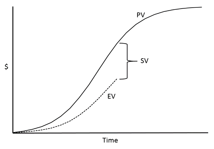 | Figure 1. Graphical representation of SV |
The schedule performance (SPI) is computed using the following equation: | (1) |
The project is ahead of schedule when SPI is larger than 1, and behind schedule when smaller than 1. These concepts have been brought to attention by books on project management and control in general [4-6] (Archibald and Villoria, 1967; Cleland and King, 1988; Kerzner, 2013) and EVM in particular [7-9] (Anbari (2003; Fleming and Koppelman, 2005; Vanhoucke, 2010a). Moreover, a comprehensive bibliography on the earned\value literature has been constructed by Christensen [10] (2015). The critics of EVM claim that the government-led centralization and lack of practitioners’ understanding of the EVM system hindered the widespread use of EVM [11] (Kemps 1993). However, the increased exposure of EVM and gradual use one practitioners led to general acceptance of the EVM system [12] (Brock 1983). Nevertheless, EVM still has some limitations that led most practitioners to regard EVM as solely a cost management tool [13] (Henderson and Lipke 2006). These limitations resulted in what Lipke described as flawed indicators [14] (Lipke 2005). To investigate the limitations of the EVM schedule indicators, a comparison to the more grounded metrics of the Critical Path Method (CPM) had to be conducted. CPM is a mathematically-based schedule network analysis technique to determine the critical paths and hence the project duration. CPM is more direct measure of time/schedule performance that consists of simple addition of activity durations to determine an overall duration. Because of the inherent calculations difference between EVM and CPM, situations could exist where the two methods provide conflicting information. For instance, if a schedule was gaining progress on non-critical, heavily weighted activities in EVM (relatively large budgets with short durations), EVM would show large amounts of progress while CPM would not show any. Erroneous information would potentially jeopardize a project, as it may misdirect leadership into making incorrect decisions.
2. Simulation Construction and Calculation
To investigate potential conflicts between SPI and CP, a simulation was created in lieu of studying existing project data. Potentially large pools of data were necessary to isolate SPI and CP conflicts, which was more difficult to organize and digest with existing data. The simulation generates project schedules and calculates the CP and SPI for each time interval within the project. It then subsequently identifies cases where CP and SPI provide conflicting information.The simulation handles projects with nine, eighteen, or twenty-seven activities. When the simulation is run, the first bits of information generated are the activity relationships (i.e.: predecessors and successors), as well as the budgeted cost and planned duration of each activity. Activity relationships are randomized every several runs, and budgeted costs and planned durations are random integer values assigned with every run. With this information, the simulation calculates the PV for each time interval. PV is calculated using the following equation: | (2) |
In Equation 2, the “Planned % Complete” is equal to the inverse of the planned activity duration. This calculation is performed for each activity at each time interval, and the total PV for each time interval (designated as PV# where # is the time interval number; e.g. “PV8” is the PV of the 8th time interval) is the sum of all planned activities that occur in the interval as seen in Figure 2. Cumulative PV will be used as the project baseline, which is the current time interval PV added to all preceding time interval PVs.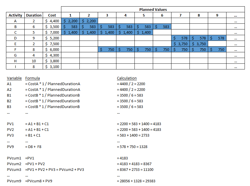 | Figure 2. Example Calculation for Planned Value at Time Interval 9 (PVcum9) |
The simulation handles the CPM by determining the Early Start, Early Finish, Late Start, and Late Finish (ES, EF, LS, LF respectively) of each activity by calculating the forward and backwards pass of the network. As seen in Table 1, to calculate the planned critical path duration, the ES of activities without predecessors is 0 (ES=0). From the ES, EF, LS and LF, the free float (FF) and total float (TF) for each activity is calculated via Equations 3 and 4, and activities that are critical (TF = FF = 0) are identified as such. From this, the EF of the last critical path activity is the planned critical path duration (notated as CP0). | (3) |
 | (4) |
Where: ESsubsequent = Early Start of subsequent activity or activities.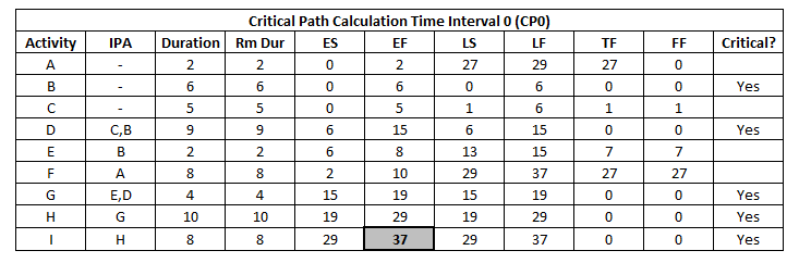 | Table 1. Example Calculation for Planned Critical Path Duration (CP0) |
Once the planned values and planned critical path duration are calculated, these values are set aside and the simulation begins to generate the remaining project data. The simulation randomly selects actual activity durations normally around the planned durations, with a standard deviation equal to 25% of the planned duration and a floor of 1 to prevent any possibility of negative activity durations. Table 2 shows a typical simulation output with the actual activities overlaid beside the plan.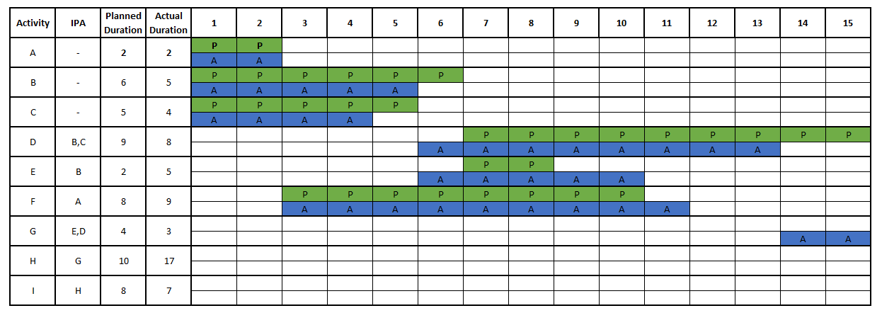 | Table 2. Example simulation output project schedule with actual activity durations versus their planned durations |
With the actual durations determined, the simulation calculates the Earned Value (EV) and the critical path duration at each time interval. EV is calculated using the following equation: | (5) |
In Equation 5, the “% of Work Completed” is equal to the inverse of the actual activity duration. Similar to the PV, this calculation is performed for each activity at each time interval, and the total EV for each time interval (notated as EV# where # is the time interval number; e.g. “EV8” is the EV of the 8th time interval) is the sum of all activities that were worked in the interval as seen in Figure 3. After the time interval EV is found, the cumulative EV is summed such that it can be compared with the cumulative PV baseline.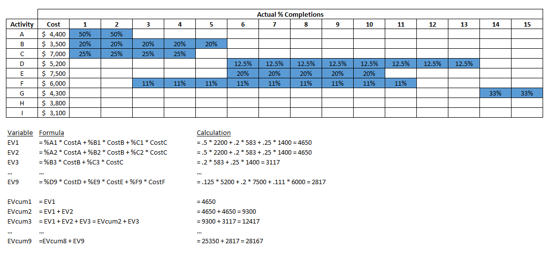 | Figure 3. Example Calculation for Earned Value at Time Interval 9 (EVcum9) |
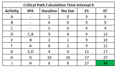
With the cumulative EV and PV calculated at each time interval, the SPI is then calculated via Equation 1 in Figure 4. From the interpretation earlier, when the SPI is >1, the project is ahead of schedule, and vice versa, for SPI <1, the project is behind schedule. In the example, SPI for the first three time intervals indicate that the project is ahead of schedule, but the SPI for the ninth time interval indicates that the project is behind schedule.Additionally for the critical path calculation, at each time interval (ES = time interval), ES, EF, LS, LF are calculated, but unlike the planned critical path duration, actual and remaining durations are used for complete and in-progress activities respectively. In Table 3, the CP duration at time interval 9 for the sample project is shown. The remaining durations are determined by referencing the output in Table 2. For example, in Table 2, in time interval 4, activities A, B, and C have remaining durations of 0, 1, and 0 respectively. At this time interval, activities A and C are complete so their remaining durations would be 0. On the other hand, activity B is only 80% complete and has one time interval’s worth of work left remaining. Because the Critical Path Duration at Time Interval 9 (value 35) is less than the planned Critical Path Duration (CP0 = 37), the project is planned to be completed ahead of schedule as of the ninth time interval.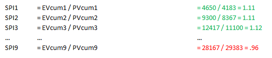 | Figure 4. Example Calculation for Schedule Performance Indicator at Time Intervals 1, 2, 3 & 9 |
Table 3. Example Calculation for Critical Path Duration at Time Interval 9
 |
| |
|
The final stage of the simulation determines whether or not the given project has conflicting schedule indicators. Before determining whether or not there are conflicting schedule indicators, the simulation automatically ignores SPI and CP calculations for all time intervals less than 7, as well as the last 20% or the last 5 time intervals whichever is greater (Lipke 2003). As discussed earlier, the very nature of SPI lends itself to misdirection around the beginning and end of the project, as it always diverges from 1 at the start of the project and converges to 1 at the end. Using the current example project schedule, the SPI at time interval 9 is <1, indicating that the project is behind schedule. Meanwhile, the CP at the same time interval indicates that the project is ahead of schedule. Because the two indicators provide conflicting information, the simulation would subsequently stop so that the project data can be observed more closely.
3. Simulation Output Examples
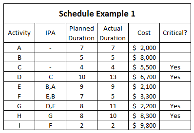
Certain project characteristics were present in projects that yielded conflicting SPI and CP. Specific sample examples of these types of projects are highlighted in this section. Additional examples and data are located in the Appendices. In the first schedule example, the simulation identified a major discrepancy between SPI and CP. Table 4 summarizes this simulation run schedule data.Table 4. Example 1 schedule Data
 |
| |
|
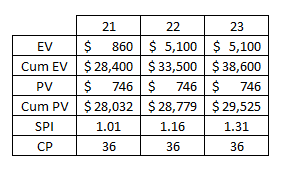
As highlighted in Table 5, the discrepancies between SPI and CP were during time intervals 22 and 23, where the SPI jumped from 1.01 at time interval 21 to 1.16 and 1.31 at time intervals 22 and 23 respectively. On the other hand, the critical path duration remained at 36, versus the planned critical path duration of 32. Looking deeper into this example, the values for EV over this time period are quite telling. There is a large increase in EV that caused the large increase in SPI: EV21 is $860, while EV22 and EV23 are both $5,100. To put this in perspective, the average EV in a time interval for this project is $1,261. During time intervals 21 through 23, the only activities that undergo any progress are activities F, G, and I. The apparent EV spike is due to the beginning and completion of activity I. As seen in Table 4, Activity I is more “dense” compared to the other activities in the project in the sense that it has a shorter planned duration than most activities, while also having a relatively large cost. To determine and compare EV activity densities, the actual duration is divided by the budgeted cost. For activities F, G, and I, this yields $660, $200 and $4,900 respectively. Intuitively, denser activities are expected to have a greater influence on EVM metrics, as EVM is solely cost-based. This, paired with the fact that activity I is non-critical. produces the situation seen in this project: large amounts of progress being reported through EVM, but no improvement of the project end date.Table 5. Example 1 schedule results at Time Intervals 21, 22, 23
 |
| |
|
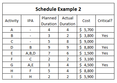
In this false positive SPI example, if the project manager were to rely on SPI, they are led to believe that their project is doing well, when in fact they are behind schedule. This type of error is particularly dangerous for a project, as corrective actions against schedule creep should typically be made in an expeditious manner.In this second example, the simulation identified the opposite discrepancy: SPI is showing the project is behind schedule, while CP shows the project is ahead of schedule. Table 6 summarizes the project data.Table 6. Example 2 schedule data
 |
| |
|
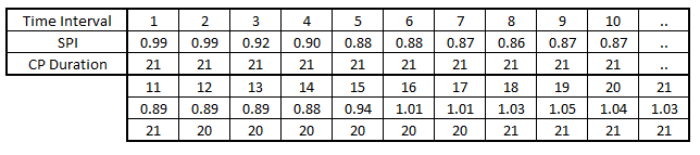
In Example 2 Schedule, the SPI lingers below .90 for most of the life of the project. On the other hand, the critical path for most time intervals is either 21 or 22, compared to the planned critical path duration of 22 (see Table 7). In this example, the SPI is indicating that the project is behind schedule, but the critical path indicates otherwise. In Table 6, most activities’ actual durations are within one day of their planned durations, with the exception of Activity C. Compared to all other activities, activity C has the largest budgeted cost, and therefore has the largest pull on the EV of the project. It is important to note that this activity is also non-critical, and therefore does not have any impact on the critical path of the project. Because this activity progresses slowly compared to the plan (8 days actual versus the 5 day plan), this activity gains little EV progress, and in turn, decreases the SPI. In the meantime, because the critical activities B and E are progressing faster compared to the plan, the critical path is shortened, compared to the planned critical path duration.Table 7. Example 2 schedule SPI and CP results
 |
| |
|
In this false negative SPI example, if the project manager were to rely on SPI for decision making, they are led to believe that their project is doing poorly, when in fact they are ahead of schedule. This type of error is somewhat dangerous, as the project manager may be inclined to spend resources of activities to speed them up, when in fact, no action is necessary.In both examples, it appears that non-critical activities with larger budgeted costs pull the EV and SPI one direction, while not making the same impact on the critical path. To determine if there is a statistically significant difference in cost between non-critical activities and critical activities at time intervals with conflicting SPI and CP, a paired t-test was performed. Data were collected from 100 time intervals where SPI and CP showed conflict. At each of these time intervals, the average cost of critical path activities and of non-critical path activities was recorded, and their difference was calculated such that a positive difference indicated that the average cost of non-critical activities was larger than the cost of critical activities. The standard deviation and mean of the differences were 1630 and 866 respectively. The following paired t-test was performed with this information: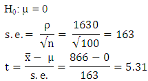 tcrit = 1.98 @ 5% confidence with d.f. = n – 1 = 100 – 1 = 99Because t > tcrit, the null hypothesis is rejected. With 95% confidence, there is enough evidence to conclude that a positive difference in the cost of non-critical path activities versus critical path activities exists.
4. Mitigation
The simulation output examples showcase scenarios where Earned Value gains progress at a different rate than Critical Path, resulting in discrepancies between the two metrics. Critical Path duration calculations rely solely on the summation of critical activity durations, and thus does not allow for flexibility in its calculation. Earned Value Management however, is derived from costs and durations of both critical and non-critical activities, allowing more flexibility in its calculation compared to Critical Path. Through fundamental analysis of EVM and CP, the following techniques can be used to mitigate discrepancies between earned value and critical path.In the following examples, a “Critical Path Equivalent” or “CPe” is calculated as: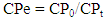 | (6) |
Where CPt is the critical path duration at a given time period and CP0 is the planned critical path duration. This Critical Path Equivalent provides a parallel metric to SPI (i.e. >1 is ahead of schedule, <1 is behind schedule, 1 is on schedule). To see the effects of the following mitigation techniques on SPI and CPe had on the full schedule, a graph of SPI and CPe at each time period was produced by the simulation. Figure 5 shows the following flow chart of the process in which the simulation generates this graph.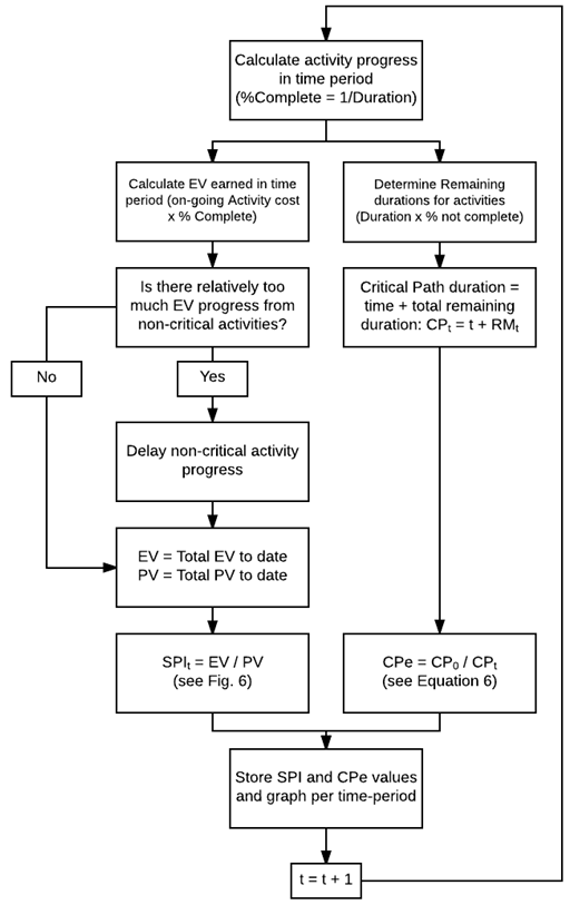 | Figure 5. Flowchart showing simulation’s process to generate SPI and CPe and chart on graph |
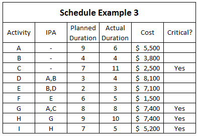
As stated earlier, earned value management is based on time and costs. The time an activity’s value is earned directly impacts the earned value at a given time period. By delaying the start of some non-critical activities, discrepancy occurrence between EVM and CP can be mitigated.Table 8. Example 3 schedule data
 |
| |
|
In Figure 6, a comparison of SPI to CPe for all time periods in Example 3 schedule. In the example given in Table 8, non-critical Activity D, which has a relatively large cost per day, causes the SPI to ramp up from T=6 to T=9 as seen in Figure 6. This early gain in earned value causes the SPI to be much larger than 1, indicating that the project is far ahead of schedule throughout the duration of the project; however, according to the CPe in the same timeframe, the project is actually behind schedule. By delaying progress on some non-critical activities, the SPI and CP align better in diagnosing project schedule health, as seen in Figure 7.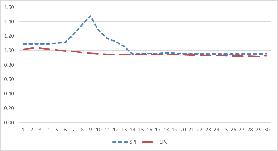 | Figure 6. Example 3 schedule SPI and CPe values |
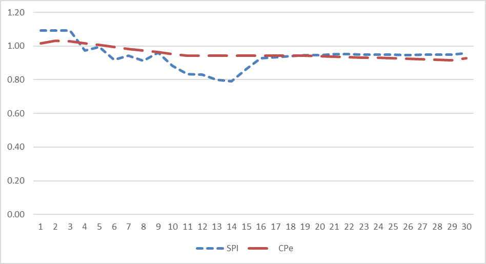 | Figure 7. Example 3 schedule SPI and CPe values after delaying non-critical activity D |
After delaying progress on certain non-critical activities, SPI and CP point in the same direction, at almost the same degree of deviation from 1. By delaying non-critical activity progress, we ensure a more steady EV gain, which in turn helps prevent large increases and decreases in SPI.Another discrepancy mitigation technique is to reduce outliers in costs per time period. In the example in Figure 7, Activities I, S, W, and X were identified as outliers in the simulation, and their overall costs were reduced to bring their Reduced Cost/day down to within Q3 + 1.5 * IQR. Cost per day was identified as a greater factor in large increases or decreases in SPI versus simply activity cost. For example, Activity C has a cost of $9,000, and an Activity A has a cost of $3,100, although activity C clearly has a greater pull on EVM metrics overall due to its larger cost, because Activity A has a much shorter duration that Activity C, the instantaneous effect on EVM metrics of Activity A is much greater than that of C ($1,550/day versus $818/day). This instantaneous effect is more likely to cause large increases and decreases in earned value, and thus SPI, and this can be especially disastrous when non-critical activities cause large gains or deficits. Project schedules are always going to have activities that weighed heavily in EVM-space and should be accepted as such, however, statistical outliers in cost per day should be identified and tracked, as they have potential to skew EVM metrics.According to Table 9, the non-critical Activity S occurs four days earlier than expected, which, coupled with its exceptionally large cost/day, results in large gains in EVM, but no progress in terms of CPM.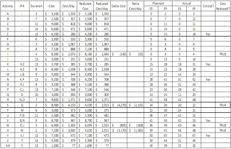 | Table 9. Example schedule activity cost/day pre- and post-reduction, highlighting Activity S |
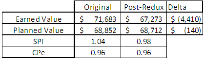
The calculations in Table 10 highlight the changes in EV and PV due to cost reduction of Activity S. The first item to note is the discrepancy between SPI and CPe. Originally, at T=23 of the schedule, SPI and CPe do not agree in schedule health. In Table 10, the $4,410 difference between original EV and Post-Reduction EV is the combined cost reduction in Activities I and S (as they are the only two cost-reduced activities to have occurred by T=23). The $140 difference between original PV and Post-Reduction PV is attributed only to Activity I, as at T=23, Activity S was not planned to start yet. Due to the relatively larger decrease in EV versus the decrease in PV, the Post-Reduction SPI is less than the original SPI to the point that it no longer shows a discrepancy from CPe.Table 10. EV, PV, and SPI Calculations for pre- and post-reduction of activity cost/day at T=23
 |
| |
|
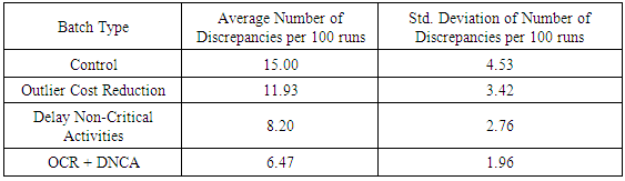
By delaying progress in non-critical activities and reducing outlier costs/day, there is an overall decrease in the number of EVM to CPM deviation occurrences. The simulation was configured to output 60 batches, 15 batches for each scenario in Table 11. In each batch, the simulation ran 100 times each, for a total of 6,000 runs, or schedules, of data. The number of discrepancies per 100 runs was recorded, and the averages and standard deviations of each are recorded in Table 11. In the simulation, a discrepancy occurrence in EVM and CPM is defined as a schedule where more than 2% of time periods after T=7 and before the last 10% of the schedule show a discrepancy in schedule health as reported by SPI and CPe [2] (Lipke 2003). Additionally, a threshold for what is considered “on schedule” is built into the simulation. An SPI or a CPe within .01 of 1 is considered “on schedule”, and any deviation greater than .01 is considered “ahead” or “behind” schedule.Table 11. Mitigation methods and their number of discrepancies per 100 runs
 |
| |
|
By comparing each batch type versus the control via a two-variable unpaired t-test with H0 = 0, we find that both the Outlier Cost Reduction method and the Delay of Non-Critical Activities show a statistically significant difference in mean values. However, if the two methods are combined, there is an extremely statistically significant difference in the number of occurrences from not using any mitigation method.
5. Conclusions
Although Earned Value Management has gained widespread use in monitoring project costs and budget, instances of EVM’s schedule metrics reporting misleading information have been isolated and analyzed. The very nature of SPI being a cost-driven metric makes it a confusing schedule indicator, especially compared to the more intuitive CPM. The results of this study have shown that projects with activities that are non-critical, but weighted heavily in EVM, SPI not only can report with inaccuracy, but can indicate a completely different direction than the critical path. This in turn can sway project decision makers to make an ill informed decision and harm the health of the project. However, by implementing both mitigation methods outlined in this paper (Outlier Cost Reduction and Delaying Non-Critical Activities), the odds of discrepancies occurring between CPM and SPI can be significantly reduced.
References
| [1] | Corovic, R. (2006). Why EVM is not good for schedule performance analysis (and how it could be…). The Measurable News, winter, pp. 22-30. |
| [2] | Lipke, W. (2003). Schedule is different. Measurable News 31, pp. 31-34. |
| [3] | Vandevoorde, S. and Vanhoucke, M. (2005). A comparison of different project duration forecasting methods using earned value metrics. International Journal of Project Management, 24 (4), pp. 289-302. |
| [4] | Archibald, R., Villoria, R. (1967). Network-based management systems (PERT/CPM), Information Sciences Series, John Wiley & Sons. |
| [5] | Cleland, D.I., King, W.R. (1988). Project Management Handbook, Second Edition, John Wiley & Sons. |
| [6] | Kerzner, H.R. (2013). Project Management: A Systems Approach to Planning, Scheduling, and Controlling, 11th edition, John Wiley & Sons. |
| [7] | Anbari, F. (2003). Earned Value Project Management Method and Extensions. Project Management Journal, 34 (4): 12-23. |
| [8] | Fleming Q.W. and Koppelman, J.M. (2010). Earned Value Project Management, 4th edition, Project Management Institute. |
| [9] | Vanhoucke, M. (2010a). Using activity sensitivity and network topology information to monitor project time performance, OMEGA International Journal of Management Science, 38, pp. 359–370. |
| [10] | Christensen, D.S. (2015). Earned value bibliography Retrieved June 3, 2015, from http://www.evmlibrary.org/search.asp. |
| [11] | Kemps, RR. (1993). Performance analysis: earned value and its pitfalls. The Measurable News. 1993, Dec: 1-6. |
| [12] | Brock, R. (1983). Earned value: burden or benefit? The Measurable News. 1983, Sept: 12-13. |
| [13] | Henderson, K. and Lipke, W. (2006). Earned Schedule: An Emerging Enhancement to Earned Value Management. Cross Talk: 26-30. |
| [14] | Lipke, W. (2005). Connecting Earned Value to the Schedule. Crosstalk. |

 Abstract
 Reference
 Full-Text PDF
 Full-text HTML