-
Paper Information
- Paper Submission
-
Journal Information
- About This Journal
- Editorial Board
- Current Issue
- Archive
- Author Guidelines
- Contact Us
International Journal of Construction Engineering and Management
p-ISSN: 2326-1080 e-ISSN: 2326-1102
2019; 8(2): 37-45
doi:10.5923/j.ijcem.20190802.01

Delay in Pipeline Construction Projects in the Oil and Gas Industry: Part 2 (Prediction Models)
 Abstract
 Reference
 Full-Text PDF
 Full-text HTML
Reyadh M. M. Mohammed, Saad M. A. Suliman
Department of Mechanical Engineering, University of Bahrain, Kingdom of Bahrain
Correspondence to: Reyadh M. M. Mohammed, Department of Mechanical Engineering, University of Bahrain, Kingdom of Bahrain.
| Email: |  |
Copyright © 2019 The Author(s). Published by Scientific & Academic Publishing.
This work is licensed under the Creative Commons Attribution International License (CC BY).
http://creativecommons.org/licenses/by/4.0/

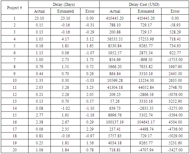
In part 1 of the paper, factors causing delay in pipeline construction projects in the oil and gas industry in Bahrain were identified and ranked based on their importance and frequency. Risk assessment of 47 critical delay factors was conducted based on a survey and XYZ Company’s KPI. In this part of the paper, delay prediction models were developed using multiple linear regression modelling. The multiple linear regression analysis was performed through the Statistical Package for the Social Sciences (SPSS) version 23 using historical data for 80 delayed oil and gas pipeline construction projects. Of the 47 critical delay factors, nineteen were considered high risk according to the risk assessment analysis. Prior to undertaking the analysis, the data was divided into two sets. The first set was comprised of 80 delayed projects for the model development whereas the second set was comprised of 20 delayed projects that were used for the model validation. The delay in days and the cost of delays were estimated using the developed models. Validation of the models showed that the model used for predicting the project costs of delays had a greater accuracy compared to the model used for estimating the project duration delays.
Keywords: Prediction models, Project planning, Pipeline construction project, Construction delay, Cost of delay
Cite this paper: Reyadh M. M. Mohammed, Saad M. A. Suliman, Delay in Pipeline Construction Projects in the Oil and Gas Industry: Part 2 (Prediction Models), International Journal of Construction Engineering and Management , Vol. 8 No. 2, 2019, pp. 37-45. doi: 10.5923/j.ijcem.20190802.01.
Article Outline
1. Introduction
- Part 1 of this paper focused on the delay factors and their risk assessment. However, development and validation of prediction models for delay was considered the most critical part of the study. Hence the study adopted the multi linear regression methodology to develop models that can be used by different stakeholders in the pipeline construction in oil and gas industry to predict the delay in days and also the cost overrun caused by the delays. Delay in the pipeline construction projects will automatically escalate the construction cost. The various stakeholders in the industry have in past strategized measures to enable completion of the project within the schedule. However, despite the positive interventions, most of the projects experience significant delays which can be otherwise avoided or reduced significantly by deploying prediction models. With the regression models, it is possible to visually examine the relationship existing between the dependent variables which are the cost of delay and the duration of delay in days, in one hand and the independent variables, which are the delay factors, in the other hand. The main objectives of this paper is to develop and validate models that can predict duration of delay in days and the cost of delay in USD.
2. Literature Review
- El-Kholy (2015) carried out a study on two models for predicting cost overruns in construction projects; Case Based Reasoning (CBR) and regression model. The study conducted a comparison of the two models and concluded that the regression model was more accurate than CBR. This study finding corroborated with an earlier study carried out by Dogan, Arditi and Gunaydin (2006). Dogan, Arditi and Gunaydin (2006) did a study to identify attribute weights in Case Based Reasoning (CBR) prediction model to estimate the costs in construction projects. The objective of the study was to investigate the application of the Excel sheet based CBR model of prediction through determining the effects of factor weights that were generated using three different optimization techniques. The three techniques were: counting features, gradient descent, and genetic algorithm. First of all, the spreadsheet was simulated for the study. This simulation was carried out in six steps: organizing and formatting data, calculating attribute similarities, establishing attribute weights, calculating weighted case similarities, identifying similarities of weight attributes and affiliated outputs, and calculating errors. A test was performed by populating data from a residential building construction project into a CBR Excel template. This data was from study reports investigating the cost of construction projects in residential buildings in Turkey. The data was then run and the results evaluated. The procedure was done 10 times for the test set and the best results were recorded. The findings from the study indicated that the GA-augmented CBR model was the best, with an estimated 16.23% error, followed by CBR + feature counting with 17.63% error and CBR plus gradient descent with 21.20% error. The study demonstrated the importance of CBR prediction model, especially in the performance of the attribute weights.A research carried out by Bayram (2017) investigated and validated the “Bromilow’s Time-cost model (BTC)” and “Love et al.’s Time-Floor model (LTF)” on the Turkish public building projects. This study had two objectives, namely: to check the two models (BTC and LTF) appropriateness, and also to compare the two models prediction performances in relation to project durations. The BTC model formulated project duration in terms of cost while the LTF model used both gross floor area and number. Best-fit models were used as bench mark for both BTC and LTF models during the research. The research findings asserted that BTC model is more superior to LTF model, thus concluding that cost is a more significant to both gross floor area and number in predicting construction duration. On the other hand, the proposed best-fit models in the research proposed cost, and the area and height to be vital predictors of duration in construction. This research finding corroborated to earlier research findings by Elhang and Boussabaine (1999) where they conducted statistical analysis in creating priority rating of the prompting factors. Additionally, this research provided ways on how to develop price models by use of both the cost and time factors.Maria and Georgios (2017) conducted a research using regression analysis in evaluating cost and time prediction for plethora of public works focused on urban renewal in the Thessaloniki district. Data on twelve public projects were provided by the Municipality of Thessaloniki. Moreover, Fast Artificial Neural Network (FANN) tool was used in predicting both duration and final cost of projects by using volume of earthwork as the input variable. The two approaches (regression analysis and FANN tool) facilitated project stakeholders on forecasting the project’s duration and costs hence enabling them to note any deviations from the set deadlines and budgetary allocations. Generally, the research indicated that the artificial fast neural network (FANN) had higher accuracy and efficiency in performance compared to the regression model in the case study. Additional past studies by Hezagy and Ayed (1998) on use of neural network in evaluating cost data and creation of prediction model for highway construction projects emphasized this finding. Here, developers created a model for testing sensitivity of changes in cost related parameters to determine their relative significance. Adaptive modules were incorporated in this study which allowed users to easily input data for re-optimization of the model to the future changing both internal and external project environments.Gunduz et al. (2017) used different standard statistical methods to evaluate their research outcomes on reasons why projects lagged in Qatar. The main objective of the study was to determine main causes of delays in construction projects. Literature review was used to identify eighty-three causes of delays whereas expert opinions and recommendations reduced the causes by forty-one causes leaving forty-two causes whose outcomes were analysis using standard statistical methods. Cronbach’s Alpha coefficient was used to measure internal inconsistencies of the outcomes whereas the Relative Importance Index (RII) and the Frequency Index (FI) applied on the assessment of different project delay factors. This is corroborated to the Gebrehiwet and Luo (2017) statement that, “timely project completion ranks highly as a project success metric alongside adherence to budget, satisfaction of quality standards, and conformance with benchmarks for safety.” Even though these factors appear standalone, numerous studies across diverse disciplines and industrial fields have reported relationships between these variables (Karami and Olatunji, 2017).Additionally, Michal, Agnieszka and Krzysztof (2018) also used artificial neural networks for cost estimation in their study. Noting the importance of cost estimation for success of any construction project, they estimated costs of constructing a sports field by use of artificial neural networks which they described as a multi-layer perceptron networks. Moreover, one network in the study was tailored for mapping the relationship between the total construction costs of the works and a selected cost predictor of the sports fields. Results from the study indicated a satisfactory performance of the different selected neural networks in terms of real costs and predicted costs. Therefore, this technique has two key advantages. These are: allows for cost estimation of construction works and support client decisions as they are aware of cost estimation accuracy.The importance of this paper lies in the fact that most of the previous studies did not cover the modeling of the duration of delay along with the cost of delay. The previous studies were mainly focused on the delay factors and their ranking without developing prediction models for delays. In addition to that, there was no research found to study this specific topic in Kingdom of Bahrain and precisely in pipeline construction projects. Therefore, this study is aimed to identify the causes and effects of the delay in the pipeline construction projects in Bahrain and to model the delay in terms of duration and cost based on real case studies in this field.
3. Development and Validation Delay Models
- Regression modelling Multiple linear regression analysis was performed in SPSS using historical data for 80 oil and gas pipeline construction projects and the KPI data. The data included the 19 high risk delay factors identified in part 1. Prior to undertaking the analysis, the data was divided into two sets comprising 80 and 20 projects used for the development of the model and its validation, respectively.A detailed breakdown of the 80 pipeline construction projects that suffered delays during the period 2011 through 2017, and the mapping out of the 19 high risk delay factors was performed (Tables 1 and 2). From the 80 late projects in the XYZ Company KPIs, the researcher had studied the actual reasons of delays to identify the definite causes and correlate the 19 high risk delay factors, resulted from the company’s risk assessment matrix, to the actual one by using binary analysis system as shown in Table (2), where a 1 implies presence of the factor and a 0 implies its absence. After filling the binary Excel sheet for the 80 delayed projects, the list was entered in the SPSS software for the delay predication models using the multi linear regression methodology.
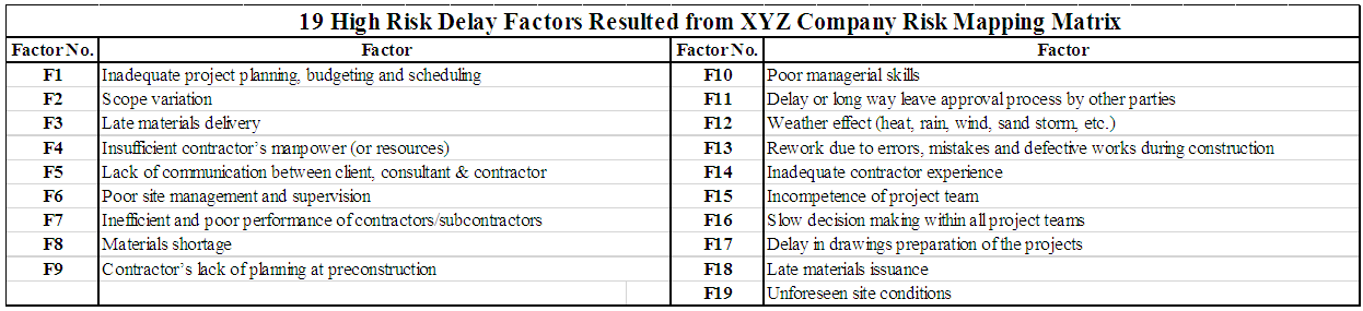 | Table (1) |
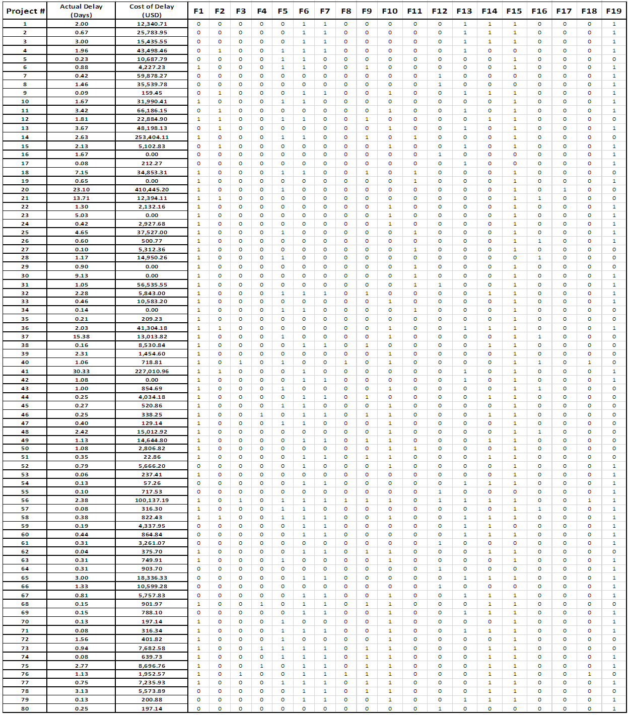 | Table (2). Binary Analysis for 80 Delayed Projects in XYZ Company using Risk Mapping Matrix Method |
 | (1) |
|

|
|
 | (2) |
|

|
|
 | (3) |
|

|
|
 | (4) |
|

|
|
|
|
|
4. Discussion
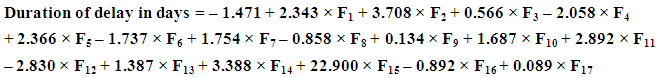
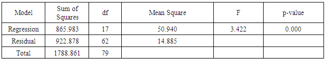
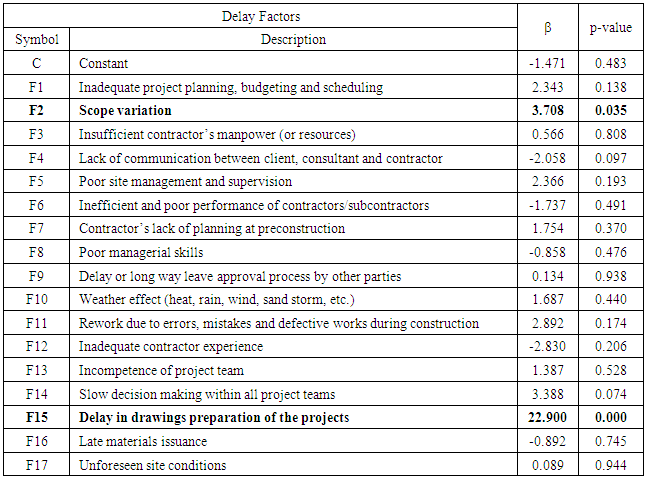
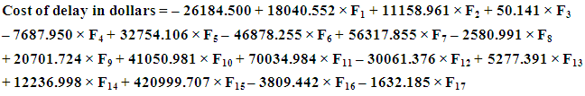
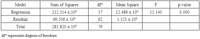
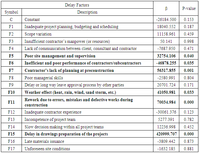
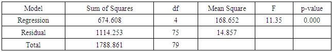
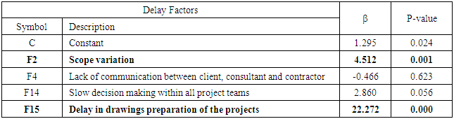
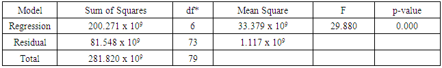
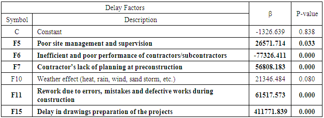
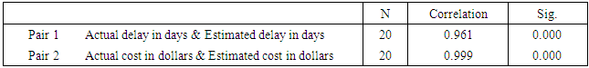
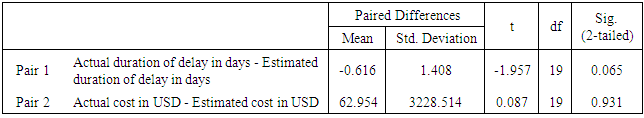
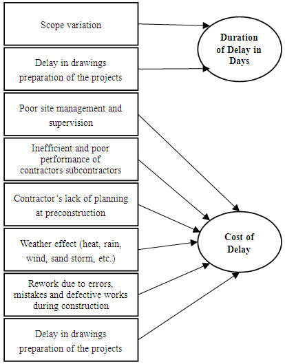
- Scope variation and delay in drawing preparations for the project emerged as important factors in predicting duration of delay. The implication of this finding was that scoping and conducting drawing preparations accurately in the project most likely would reduce the length of a project delay. On the other hand, the contractor related delay factors that affecting the cost model were: poor site management and supervision, inefficient and poor performance of contractors/subcontractors, contractor’s lack of planning at preconstruction, and rework due to errors, mistakes and defective works during construction. However, it should be noted that delay factors related to design were also significant predictors of delay costs and delay duration. The ascertainment received from the paired samples t-test and the regression test was adequate to render the models reliable. The prediction model for cost of delay revealed a higher prediction power with more significant delay variables than the model for duration of delay. The model of duration of delay had a prediction power of 34.3% while the model of cost of delay had prediction power of 68.6%. The predictive power of the project cost of delays linear regression model was emphasized by the statistical results from t-test paired two samples for mean, which indicated that the means of actual project cost of delays and the means of estimated projected cost of delays seemed to be equal. However, the results from t-test paired two samples for means indicated that the means of actual project duration delays in days seemed to be statistically different and low compared to the means of estimated project duration delays in days.Based on the two regression models for duration of delay in days and the cost of delays, Figure (1) shows the significant predictor variables for each model.
 | Figure (1). Prediction Models for Delay in Pipeline Construction Projects in Oil and Gas Industry as Developed in This Paper |
5. Conclusions and Recommendations
- The study acknowledged that based on the outcome from linear regression analysis, project scope variation and delays in drawings preparation for the project have a significant effect in predicting project duration delays. However, the factors explained only 34.3% of the variations in project duration delays. On the other hand, the analysis showed that five delay factors, namely: poor site management and supervision; inefficient and poor performance of contractors/subcontractors; contractor’s lack of planning at preconstruction; rework due to errors, mistakes and defective works during construction; and delay in drawing preparation of the projects have a significant effect in predicting cost of delay. The developed model can explain 68.6% of the variations in project cost of delays. On the basis of results from the multiple linear regression analysis, the study concluded that the project cost of delays prediction model had a greater predictive and forecasting ability compared to the project duration delays prediction model. The findings are also emphasized by the statistical results from t-test paired comparison of means in both prediction of duration delays and cost of delay. Based on the findings, the research recommends the following:Ÿ The significant model predictor variables of project duration delay can be mitigated by having additional measures at the preconstruction phase. This can be achieved by making a precise scope tender documents to avoid variations during the actual construction. In addition, the designer should be asked for clear time line for the design drawing to avoid submitting the drawing late, andŸ The significant model predictor variables of cost of delay can be mitigated by providing instant performance feedback to the contractor in a frequent basis during all project stages (planning, execution and closing out the project). Furthermore, spending more time in planning stage from client and contractor side is recommended in order to achieve the target goal with the allocated budget for the project. Some other factors effect can only be minimized and cannot be eliminated such as heat, rain, sand storm... etc. in these cases some extra precautions can be taken in order to speed up the project such as providing shades, special clothes to withstand the heat, face masks for the sand storm and regular rests and breaks for the labors. In some of the cases, the delay happens from rework in the project during construction, to avoid these kind of delays, extra and constant supervision needed on site from both parties the client and the contractor these delay have direct impact on the project duration therefore on the project cost as well.
6. Further Research
- Further research is needed on:Ÿ Enhancing the developed model in this study through introduction and testing of additional factors to enhance the prediction power of delay duration and cost in pipeline construction project in the oil and gas industry, andŸ Further research is needed to test the model using data from different companies in the same field in Bahrain and other countries pipeline industry sectors to investigate the applicability of the prediction models for other companies.