1. Introduction

Important equipment management decisions are based on estimates of owning and operating costs throughout the life of a machine. Equipment managers rely on such estimates to establish cost recovery rates, define equipment replacement cycles, develop operating cost budgets, evaluate acquisition strategies, and establish unit cost rates. Owning and operating costs are typically modelled separately and then combined to form a total cost model used by managers. The traditional model for equipment costs is the average total cost minimization model [1], where the objective is to minimize the total cost divided by the measured equipment use.

Owning costs, the costs of acquiring and keeping a machine in the fleet, are incurred irrespective of machine use. The cost transactions associated with owning a machine include depreciation charges; the costs of licenses, insurances, and taxes; the cost of capital required for acquisition; and resale of the machine at the end of life [2]. The timing and magnitude of the cost transactions are largely known at the time of acquisition, with the exception of the magnitude of the resale value. Resale value and the methods to estimate it have been addressed by Lucko and Vorster [3], Lucko et al. [4], and Lucko et al. [5].

Operating costs are incurred for every hour the machine is put to work, and include the costs of repairs, fuel, preventive maintenance, tires or tracks, and wear parts [6]. Not included in operating costs are the labor wages of the operator, or mobilization and de-mobilization costs. Most operating costs are incurred at a relatively constant rate and can be easily forecast. However, repair costs increase throughout life due to increasing frequency and magnitude of repair actions [7]. Thus, the rate at which operating costs are incurred increases with machine age and can be modelled in the same manner as repair costs.

Operating cost models are typically developed in the form of cumulative cost versus machine age in hours or miles. The appropriate selection of the method to develop such models depends on the availability of cumulative cost data and whether machine age is maintained in terms of use or years. Mitchell [8] presents techniques to regress cumulative cost on cumulative hours worked when both are known. Mitchell et al. [9] and Bayzid et al. [10] describe techniques for a period cost based analysis that can be applied when cumulative hours worked is known but cumulative cost is not. The methods described by Kaufmann et al. [11] rely on estimates of operating rates developed from machine age in years and annual data regarding cost and use to construct a cumulative operating cost model.

Operating rates calculated from annual data are inherently more variable than those calculated from cumulative data because the rates are based only on what was experienced by the machine in the year. Rates from cumulative data reflect the entire experience of the machine from the time it was initially brought into the fleet. Within annual data, overly high rates are not offset by overly low rates because operating rates are bound on the lower end and theoretically unbounded on the upper end. Therefore, it is hypothesized that operating cost models from annual data will tend to overestimate costs over the life of a machine. The objective of this research was to compare operating cost estimates developed from annual data with observed cumulative cost data to determine the extent and magnitude of overestimates from annual data.

2. Background

2.1. Equipment Operating Cost Forecasting

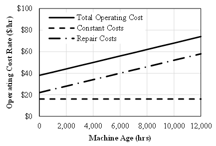
Operating costs can be broadly categorized into those costs that are incurred at a relatively constant rate and those that are incurred at an increasing rate over the life of the machine. The costs of fuel, preventive maintenance, tires or tracks, and wear parts are relatively constant as each component has a fixed cost and fixed life. For example, a set of tires may last 4,000 hours and cost $10,000 to replace yielding a constant rate of $2.50 per hour or fuel may be consumed at a rate of 6 gallons per hour and cost $4.50 to purchase and dispense yielding a rate of $27 per hour. As such costs are incurred at a constant rate, the cumulative costs are directly proportional to the hours worked.

Douglas [1] notes that the costs of repairs are incurred at an increasing rate because the frequency and magnitude of repair actions increase as the machine ages. This non-linear relationship between cumulative repair costs and age has been the subject of multiple studies. The mathematical form describing the relationship between repair costs and age can also be applied to operating costs because the form is not changed when the categories with constant costs are included. This is easiest demonstrated by considering the relationship between operating cost rate and machine age, as shown in Figure 1. The form of the total operating cost rate is the same as that of the repair cost rate.

Figure 1. Relationship between Operating Cost Rate and Machine Age

2.2. Estimating Repair Costs

While the rate of repair costs is widely recognized to increase with machine age, the variety of estimating methods employed include those that assume the rate is constant. In such methods, repair costs have been estimated as a percentage of capitalized value [12], annual ownership costs [13], or depreciation [14]. Terborgh [1] theorized that repair costs increase over the life of a machine and are related to accumulated use. Most methods for estimating repair costs follow this theory and equipment manufacturers have supported the use of modified straight-line approaches for establishing repair reserves [15, 16, 17]. Nichols and Day [14] present a methodology for estimating the repair cost rate that includes a set of factors that increase with accumulated use and are applied to adjust a constant repair rate calculated as a percentage of the purchase price.

2.2.1. Estimating Based on Measured Equipment Use

Historical cost records are the reliable dependable means for estimating repair costs [18]. Mitchell [8] applied regression techniques to field data to evaluate model forms and determine the best fitting model to represent repair costs in terms of machine age in hours of use. Cumulative repair cost and use data were collected for 260 machines operating in 17 different fleets managed by four construction companies. The best fitting model was the second-order polynomial:

(1)

Where:

CC_RPL = cumulative cost of repair parts and labor from 0 hours to H_w hours;

H_w = life to date hours worked by the machine; and

A and B are coefficients.

This model is known as the Mitchell Curve and is widely used by equipment managers. Repair costs are accrued, in part, directly proportional to the hours worked and is reflected by the A coefficient. The increasing rate of repair cost accrual as the machine ages is reflected by the B coefficient. Costs associated with maintenance and actions that prevent machine failures contribute to the A coefficient, while repair actions resulting from failures contribute to the B coefficient [19].

The advantages of the Mitchell Curve methodology are that the results are based on historical data collected from machines in the fleet and reflect the entire experience of the machines [9]. Machines often experience periods of good, bad, and average repair cost accumulations throughout their life and using data reflective of all experiences produces results that are both stable and representative of what can be expected. The principal limitation to the methodology is the availability of quality life-to-date data needed to drive the analysis. Life-to-date data is not available for machines purchased on the resale market, or where reliable cost data has not been maintained since purchase of a new machine.

The Period Cost Based (PCB) methodology for estimating repair costs overcomes the need for life-to-date data by making use of repair costs experienced over a fixed period defined by the machine age in hours at the start (H_s) and end (H_e) of the period to estimate the A and B coefficients of the Mitchell Curve [9]. It is based on the application of the mean value theorem to the second-order polynomial form, which results in the average cost of repairs over the period equaling the marginal cost of repairs (m) for the machine at age (H_m) midway between H_s and H_e. The PCB concept is shown in Figure 2.

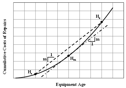Figure 2. Period Cost Based Method Concept

The marginal cost of repair costs at age H_m is given by the derivative of the Mitchell Curve with respect to H_w and evaluated at H_m:

(2)

Regressing marginal cost (m) on H_m yields the following marginal cost model with respect to machine age:

(3)

Where:

m is the marginal cost at machine age x;

K is equal to the A coefficient of the Mitchell Curve, and

V is equal to twice the B coefficient of the Mitchell Curve.

The values of A and B determined by the PCB methodology are useful for estimating cumulative repair costs throughout the life of the machine from partial equipment histories. This ability to model costs based on data from machines for which cumulative cost data is not available either because the data was not maintained or the machines were not purchased new is the primary advantage of the PCB methodology. The principal disadvantage is that period data is less stable than life-to-date data and the repair costs experienced during the period may not reflect the costs normally expected.

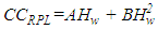
2.2.2. Estimating Based on Equipment Age

Data regarding machine age may not be available in terms of accumulated use, in which case age is measured in years. This may be the result of inaccurate hour meters due to failure or replacement, or a failure to maintain records. In any case, without machine use data the cumulative cost and PCB methodologies cannot be used to estimate repair costs. Machine age in years combined with historical cost records for the year provide annual data that can be used to model and estimate operating and repair costs.

Nunnally [2] presents a method of estimating annual repair costs based on age that is effectively the reverse of the Sum-of-Years’-Digits method typically used to calculate depreciation. Alternatively, statistical methods can be applied to records of annual operating or repair costs to develop a model of annual costs based on age. Terborgh [1] postulated the modified exponential model for estimating the average hourly repair rate (R) in relation to age:

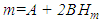
(4)

Where:

k is the asymptote to which R approaches as a limit with the increase in x;

x is the machine age in years, and

a and b are regression coefficients.

The exponential form has also been applied to model average hourly operating rate (O) in relation to machine age [11, 20]:

(5)

Where:

k is the regression coefficient representing the initial operating rate;

t is the regression coefficient representing the annual increase in operating rate, and

x is machine age in years.

Both methods produce estimates of hourly rates which must be combined with an estimate of annual use to estimate annual costs. Estimates of both annual use and cost can be made throughout the life of a machine and summed to produce cumulative models. The simplest estimate of annual use is to assume constant use throughout the life of a machine. This simplistic assumption rarely if ever reflects reality, and annual use typically declines as a machine ages. Terborgh [1] terms this decrease in annual use as functional degradation and describes the phenomena as the result of quantitative degradation and qualitative degradation. The gradual decline in annual use resulting from a machine being shifted as it ages to roles of less continual and intense use is quantitative degradation. Qualitative degradation is the gradual decline in use resulting from the loss in machine precision and movement towards roles for which the requirements are less exacting. The linear form was used to model the decreasing annual use in equipment by Kauffman et al. [11] and Kauffman et al. [20].

Annual cost and use data are highly variable because they reflect performance over a limited time period, as opposed to cumulative data that encompasses the entire history of the machine. Thus, the cost rate and annual use models rarely fit the underlying data well, as reflected by low goodness-of-fit (R²) values. Kauffman et al. [11] and Kauffman et al. [20] analyzed a large number of machines in several different equipment classes and not all models and R² values are presented. However, for the results presented for seven equipment classes, the variability in the annual operating rate and use is visibly quite large. The reported R² values range from 0.099 to 0.191 for annual operating rate and from 0.053 to 0.245 for annual use. These R² values are substantially less than the 0.72 reported by Mitchell [8] and 0.83 reported by Mitchell et al. [9] for cumulative cost models; and 0.50 reported by Mitchell et al. [9] and 0.54 reported by Bayzid et al. [10] for PCB models.

3. Research Methods

3.1. Data Source

As stated previously, the objective of this research was to compare operating cost estimates developed from annual data with observed cumulative cost data to determine the extent and magnitude of overestimates from annual data. Data regarding operating cost and use was collected for class 0314 backhoe loaders and class 0900 motor graders operated as part of a state transportation agency maintenance equipment fleet.

Annual data was collected for all of the machines in the fleet at least one year in age and for which working hours were recorded. Machines without a minimum of one full year of use were excluded because initial machine setup costs were included and are not true operating costs. Data was collected for 250 backhoe loaders and 385 motor graders, and included machine age in years, and total operating cost and hours worked for the calendar year. Machine age was the time from when the machine was brought into the fleet to the end of the year for which data was collected. The backhoe loaders ranged in age from 2.8 to 17.3 years, and the motor graders ranged from 3.2 to 21.7 years in age. The total operating cost for each machine included all costs incurred during the year for maintenance, repairs, fuel, and tires.

The recent implementation of a new data management system limited the machines for which cumulative data was available to those brought into the fleet in the last 10 years. To maximize the amount of data, selection of machines was based on the number of machines and length of operating history. Data was collected for 21 Case model 590SM2 backhoe loaders and 34 Volvo model G720B motor graders. Cumulative operating cost and hours worked were collected for motor graders 10 years in age and backhoe loaders nine years in age, as a small number of backhoe loaders were brought into the fleet 10 years prior. The data consisted of the hours worked and operating costs incurred in each calendar year of operation.

The operating cost data collected spanned a 10 year period. The Consumer Price Index (CPI) was used to adjust the annual and cumulative costs to a common basis.

3.2. Model Development

Annual data for backhoe loaders and motor graders was used to develop the following models:

Ÿ Mathematical model of average operating rate by machine age in years;

Ÿ Mathematical model of annual hours worked by machine age in years, and

Ÿ Computational model of estimated operating cost with accumulated use.

The average operating rate in the year was calculated by dividing the total operating cost by the hours worked in the year. Regression analysis was applied to fit an exponential model to data pairs of average operating rate and machine age. The models for both backhoe loaders and motor graders were both statistically significant with p-values of 3.6E-9 and 6.5E-11, respectively. The operating rate data was highly variable for both backhoe loaders and wheel loaders, as demonstrated in Figure 3, and the R² values of the models were 0.13 and 0.11, respectively. The low R² values indicate that only a small portion of the variability in operating rate can be explained by machine age, and that there are other factors besides age influencing the rate.

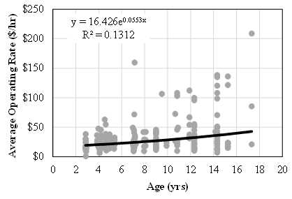Figure 3. Operating Rate by Machine Age for Class 0314 Backhoe Loaders

Regression analysis was also applied to fit an exponential model to data pairs of annual hours worked and machine age. The models for both backhoe loaders and motor graders were both statistically significant with p-values of 7.3E-19 and 2.0E-32, respectively. While the models fit better than those for the operating rate, there was substantial variability in the data as demonstrated in Figure 4. The R² values of the models for backhoe loaders and motor graders were 0.27 and 0.31, respectively.

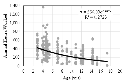Figure 4. Annual Hours Worked by Machine Age for Class 0314 Backhoe Loaders

Computational models were developed for backhoe loaders and motor graders to estimate operating costs as a machine accumulates use. On a year-by-year basis, the estimated operating cost is the product of the average operating rate and annual hours worked estimated from the mathematical models developed.

The models were evaluated at the mid-point of a machine’s age to estimate the rate and hours worked throughout the year. For example, an age of 2.5 years was used in the third year of machine life to reflect the change in age from 2 at the beginning of the year to an age of 3 at the end of the year. The computational model for backhoe loaders is provided in Table 1.

Table 1. Computational Model of Operating Costs with Accumulated Use for Class 0314 Backhoe Loaders

The observed cumulative data was used to develop mathematical models of operating cost with accumulated use in the form of the Mitchell curve for backhoe loaders and motor graders. Regression analysis was applied to the cumulative hours worked and total operating cost recorded at the end of each year. Thus, each of the 21 backhoe loaders contributed nine data points, and the 34 motor graders each contributed 10 data points to the respective models. The resulting models and parameter values were tested and found to be significant at the 0.05 level of confidence. The models fit the data well and produced very high R² values of 0.97 and 0.95 for backhoe loaders and motor graders, respectively. The data and Mitchell curve produced for backhoe loaders is presented in Figure 5.

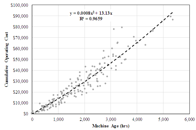Figure 5. Observed Operating Costs and Mitchell Curve for Class 0314 Backhoe Loaders

4. Results and Discussion

4.1. Comparison of Estimated Operating Costs from Cumulative and Annual Data

The results obtained for both backhoe loaders and motor graders support the hypothesis that operating cost models developed from annual data tend to overestimate operating costs over the life of a machine. As shown in Figures 6 and 7, the operating costs for both backhoe loaders and motor graders estimated from annual data were consistently greater than those represented by the Mitchell curves developed from cumulative data. While both reflected the accrual of operating costs at an increasing rate, the estimates from annual data increased at a greater rate. For backhoe loaders, operating costs were overestimated by 18 to 27 percent when compared to the Mitchell curve at the same age. Similarly, overestimates for motor graders ranged from 22 to 41 percent.

When compared to the observed operating costs, it was apparent that the costs estimated from annual data were not beyond possibility. However, they were reaching the limits of reasonable probability. As shown in Figures 6 and 7, the estimated operating costs were at or near the highest edge of the envelope encompassing the actual costs incurred. It is important to note that estimated costs represent expected costs as machine use accumulates. As such, it is anticipated that actual costs would be both higher and lower, but centered upon the expected costs. The computational models used to develop the estimated costs does not yield a true average value. Thus confidence intervals for the estimated costs cannot be calculated.

Operating costs are overestimated when based on annual data due to the increased influence of high average operating costs rates for individual machines within a single year. The high rate for a machine may accurately reflect machine performance in the year, but its influence on the estimated costs is increased due to one or both of the following:

1. The nature of costs, and by extension cost rates, is that effects of high costs are not offset by low costs. There is a real minimum cost and the maximum cost is largely unbounded. As applied to equipment operating costs, the minimum cost is at least the cost of the fuel, and likely includes preventive maintenance and other costs. The maximum cost is theoretically unbounded, but practically not so. Significant repairs can result in operating costs that are orders of magnitude greater than costs for the average machine of the same age. Such repairs also limit the hours worked, which magnifies the difference in terms of operating rate.

2. When modeling with annual data, a high cost rate is considered and incorporated into the model without knowledge or consideration of machine history. The annual data provides a snapshot of the cost situation, or an “instantaneous” cost rate of sorts. Whereas cumulative data provides and makes use of the average life-to-date cost rate that reflects periods of both high and low cost rates throughout the machine history.

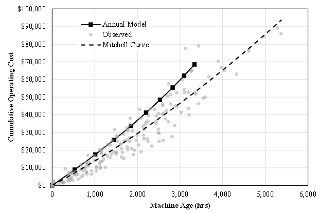Figure 6. Estimated and Observed Operating Costs for Class 0314 Backhoe Loaders

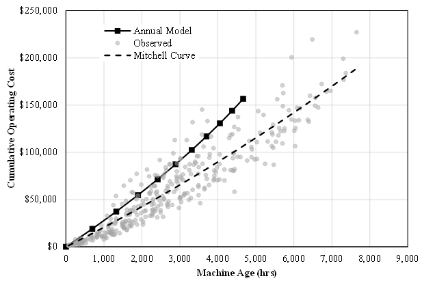Figure 7. Estimated and Observed Operating Costs for Class 0900 Motor Graders

4.2. Implications of Overestimating Operating Costs

Equipment managers use estimates of operating costs in a variety of decision making processes, but most significantly in setting cost recovery rates and establishing equipment replacement cycles. Overestimating operating costs adversely impacts the results of both processes and leads to higher than necessary rates and over recovery of costs, as well as shortened replacement cycles.

A state transportation agency maintenance equipment fleet, such as that from which the data was collected, and the equipment fleets for most private construction companies are not managed to be a profit center. Rather, the objective is to recover the costs incurred by charging projects for each hour a machine is worked. The rates are established by carefully considering the costs expected to be incurred, and overestimates of operating costs then lead to rates that over recover costs. While over recovery may initially appear as positive outcome, particularly when compared to under recovery of costs, it is the result of overcharging projects for the equipment.

It is the overcharge for equipment that may result in detrimental impacts. Within a competitive bidding environment, overcharging for equipment reduces price competitiveness. Additionally, the reputation of and support for equipment management and managers may suffer within an organization. This can lead to the development, continuation, and/or increase in strained relationships between equipment management and operations management. If the overcharge is sufficiently large, then those responsible for field operations and costs may turn to short-term rentals to equip projects at a lower cost. This can, in turn, lead to utilization problems throughout the fleet.

It is the increase in operating costs, and specifically repair costs that leads to replacing an older machine with a newer one. Overestimating operating costs, and the rate at which they are expected to be incurred, leads to underestimating equipment replacement cycles. Replacing equipment before it is cost effective results in increased capital requirements and financing costs.

5. Conclusions

The objective of this research was to compare operating cost estimates developed from annual data with observed cumulative cost data to determine the extent and magnitude of overestimates from annual data. Mathematical models of operating cost rate and annual hours worked were developed with respect to machine age and used to construct a computational model of cumulative operating cost as a machine accumulates use. The results obtained support the hypothesis that operating cost models developed from annual data tend to overestimate operating costs over the life of a machine. Estimates from annual data were consistently higher than recorded costs and the magnitude of the overestimate in costs ranged from approximately 20 to 40 percent as compared to estimates from cumulative cost records.

The magnitude of the overestimate in operating costs is substantial and may lead to decreased price competitiveness, strained relationships within management, and decreased equipment utilization. However, most surprising was that the operating costs estimated from annual data were within the envelope of cumulative cost records, albeit at the upper edge. This leads to the conclusion that estimating operating costs from annual data is a viable methodology in the absence of all other data. The methodology benefits from its basis on data that reflects actual operating conditions, maintenance and repair procedures, and management processes. The resulting estimates can be viewed as accurate, if not precise. The resulting estimates can be useful in developing baseline parameters for managing equipment until they can be refined based on more precise data.

The results underscore the importance of accounting for machine age in terms of hours worked rather the years in the fleet. Operating costs, by their very nature, are incurred for every hour the machine is worked and not simply with the passage of time. The considerable variability in the operating rate and annual use data present when machine age is accounted for in years is passed onto and compounded within the computation model of operating costs with accumulated use.