Sean (Saeed) A. Pour1, H. David Jeong2, Tieming Liu3, Garold D. Oberlender4
1Hazen and Sawyer, Irvine, CA, United States
2Department of Civil, Construction, & Environmental Engineering, Iowa State University, Ames, IA, Unite States
3School of Industrial Engineering and Management, Oklahoma State University, Stillwater, OK, United States
4School of Civil and Environmental Engineering, Oklahoma State University, Stillwater, OK, United States
Correspondence to: H. David Jeong, Department of Civil, Construction, & Environmental Engineering, Iowa State University, Ames, IA, Unite States.
| Email: |  |
Copyright © 2015 Scientific & Academic Publishing. All Rights Reserved.
This work is licensed under the Creative Commons Attribution International License (CC BY).
http://creativecommons.org/licenses/by/4.0/

Abstract
In price-time bi-parameter bidding (A+B bidding), the owner has to calculate unit time value (UTV) before letting projects because contract time must be converted into dollar value. This study investigates the impacts of different UTVs on the competitiveness of contractors in the A+B bidding process using the entire set of historical A+B bidding projects completed in Oklahoma. The study clearly shows that different UTVs do change the competitiveness of contractors during the bid process for an A+B project. Based on this empirical finding, a new formula is developed to assist SHAs in quantitatively measuring the level of competition among contractors in the bid process. This study concludes that determining the UTV mainly based on expected road user costs may lead to sub-optimal performance and adjustment of the UTV by using the new formula would increase the competition among contractors and may contribute to reducing the total project time and cost.
Keywords:
Innovative contracting, A+B contracts, Bid, Highway projects
Cite this paper: Sean (Saeed) A. Pour, H. David Jeong, Tieming Liu, Garold D. Oberlender, Impacts of Unit Time Values on Bidders’ Competitiveness in A+B Highway Contracts, International Journal of Construction Engineering and Management , Vol. 4 No. 6, 2015, pp. 219-229. doi: 10.5923/j.ijcem.20150406.01.
1. Introduction
Interstate highways in the United States not only have passed their original design life, but also have carried much more traffic volume and weights than what they had been designed. According to the 2013 ASCE infrastructure report card, roads have been given a grade of D [1]. Poor highway conditions have caused transportation agencies to shift their focus from expanding road networks to rehabilitation of their existing infrastructures. Unlike new highway construction projects, rehabilitation and reconstruction projects affect the traveling public adversely due to delays in traffic flow and safety problems. In response to increasing road user costs caused by rehabilitation or reconstruction projects, State Highway Agencies (SHAs) have started to utilize innovative contracting methods by incorporating construction time into the bidding process. Traditionally, the SHAs have used the bid price as the major criterion in evaluating contractors’ proposals. In price-time bi-parameter bidding (A+B bidding) methods, however, a combination of price and construction time is considered as the decisive factor in awarding a contract to the construction contractor. The purpose of these bidding methods is to obtain accelerated construction at the lowest possible cost in order to minimize inconvenience to the public.Several previous studies in this domain have focused on optimizing the incentive/disincentive (I/D) rates with respect to road user costs [2-7]. Time-related I/D provisions are an innovative way of reducing construction duration by offering contractors an early completion incentive bonus that can motivate them to apply their ingenuity to completing projects early [8, 9]. The goal of this study is to develop a framework that would allow SHAs to evaluate the impact of unit time value (UTV) on the competitiveness of contractors in A+B bidding projects. Actual A+B bidding data from the Oklahoma Department of Transportation (ODOT) are analyzed to develop price-time relationship models for contractors. The public accessibility to this data provides an opportunity for prospective contractors to research the bidding patterns of their competitors and adjust their bidding strategy accordingly. It also provides ODOT with an opportunity to determine the price-time relationships of contractors. The framework developed in this study can be used as a new tool to determine UTV and I/D amounts more effectively in A+B contracts to increase competition and it also enables contractors to adopt more competitive strategies.There are two different A+B contracting methods: 1) A+B without I/D and 2) A+B with I/D. In both methods, the low bidder is determined from the results of the A+B procedure utilizing UTV, and the estimated project duration submitted by the successful bidder becomes the contractual project duration. In A+B without I/D contracts, the UTV is only calculated to determine the low bid, and the contractor does not receive any incentive for early completion, nor pays any disincentive for late completion other than normally specified liquidated damages. In A+B with I/D contracts, I/D rate is set equal to UTV and the winning contractor receives an incentive for early completion, or is charged a disincentive for late completion.
2. Background
In price-time bi-parameter bidding (A+B bidding), the contract duration is determined by competition during the bid process. This procurement method incorporates the value of construction time with the bid price in evaluating contractors’ total combined bid (TCB). The successful bidder is the contractor who submits the lowest TCB using the following formula: | (1) |
Where, A is the contractor’s bid price, UTV is the unit time value defined by the owner and t is construction time (contract time). Thus, there are theoretically an infinite number of combinations of (A, t) that result in the same TCB when the UTV is fixed. UTV represents the cost of delays to the owner and is calculated by the owner for every project. According to Herbsman et al. [6], UTV includes both direct and indirect costs. In the highway construction industry, UTV is commonly referred to as the daily road-user cost. A memorandum issued by the California Department of Transportation on June 12, 2000 [10] stated that although exceptions may be allowed, UTV typically ranges from 50 to 100 percent of the calculated daily road user cost. Most state highway agencies calculate the UTV and apply this value as their daily I/D fee. However, there are some states using different parameters for establishing I/D fees, such as a percentage of total project cost. Fick et al. [4] suggest that market influences, such as the number of qualified bidders and the availability of other work to contractors, should be included as significant factors in determining I/D rates. Despite the procedural variations in calculating UTV and I/D rates, SHAs agree that the incentive amount has to be more than the contractor’s additional costs for accelerating construction and less than a dollar value of total time savings in order to effectively encourage contractors to expedite construction. Time-related I/D provisions are frequently used by SHAs to minimize construction duration, especially in urban areas where inconvenience to the traveling public is a matter of importance. This method is an innovative way of reducing construction duration by offering contractors an early completion incentive bonus that can motivate them to apply their ingenuity to completing projects early [8, 9]. According to the Federal Highway Administration (FHWA), the major area of concern on the use of I/D provisions is the determination of the appropriate dollar amount per day for early completion of projects [11]. Arditi et al. [12] suggest that the use of “A+B Bidding” in association with I/D contracts and its likely impact on contract efficiency need to be further explored. They report that contract duration will be more realistic when the project duration is set by the winning bidder, compared to when it is set by the owner in I/D contracts. They also report that “A+B Bidding” competition results in the elimination of inefficient contractors. Herbsman et al. [6] also report the need to study the interactions of A+B bidding and I/D provisions. Although several studies have investigated the optimal UTVs [4, 12, 13], studies on the interactions between the UTV and competition between contractors are very limited. Shen et al. [14] model the most competitive strategy of a single contractor without considering the collective impact of other contractors’ competitive strategies on the bid process. Shr and Chen [15], on the other hand, have assumed that all contractors share a single price-time curve and suggested a methodology to determine a maximum incentive rate for A+B contracts. Thus, no study has investigated the impact of UTV on A+B bidding competition.
2.1. Total Combined Bid Iso-Map
In A+B bidding, contractors are allowed to adjust their Total Combined Bid (TCB) by trading-off contract time and bid price. As shown in Eq. (1), contractors can increase the construction duration (t) and keep the TCB constant by decreasing the original bid price (A).Since TCB is the only factor that defines the winner of an A+B bidding contract, all the bidding strategies that result in the same TCB have the same level of competitiveness. In fact, with a given UTV, there are infinite combinations of bid price (A) and contract time (t) that give the same TCB. In a price-time orthogonal coordinate diagram, these combinations form a straight line, which has been called Iso_Line by Shen et al. [14] as shown in Figure 1. The slope of the Iso-Line is determined by the UTV and since all the points on the line have the same TCB, the line is called TCB Iso-Line. Therefore, A+B bidding can be treated as a single parameter bidding by considering the total combined bid.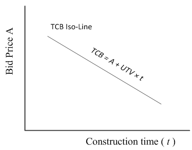 | Figure 1. Contractor’s Overall Competitiveness: TCB Iso-Line [14] |
2.2. Price-Time Function
Callahan et al. [16] report that for a specific construction company, there is an optimum price-time balancing point for every construction contract where construction cost is minimum. In general, the relationship between construction cost and time can be expressed by the curve shown in Figure 2 [17]. A bid price-time relationship can be developed by adding a certain profit margin to the construction cost.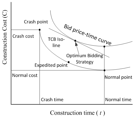 | Figure 2. Construction Cost and Bid Price Versus Time [17] |
The optimum price-time point represents the construction plan where construction cost is the lowest with a specific construction time. Shortening construction time from the optimum price-time point may require multiple shifts, overtime work, enhanced manpower and equipment, or accelerated material delivery that can increase the project direct cost. On the other hand, by extending time from the optimum price-time point the overhead costs and costs of renting equipment would increase project direct cost. As a result, the price-time curve decreases to a minimum and then increases, which is an indicator of a non-linear equation. Thus any variation in time from the optimum price-time point will result in a corresponding increase in construction cost. Several studies have suggested a quadratic or second-order polynomial function to approximate the relationship between bid price (A) and construction time (t) [13, 14, 17, 18]. | (2) |
Eq. (2) represents the second-order with three unknown constant values where A is bid price; t is construction time; and a, b1, and b2 are constant values. Shr and Chen [13], have used the actual completed project performance data and developed a single price-time curve for all contractors and incentive contracting methods (I/D with A+B, I/D without A+B, and Non Excuse Bonus projects) for the Florida Department of Transportation. After the price-time curve for a contractor is determined, the most competitive strategy is determined by finding the t in Eq. (1) that minimizes TCB. The objective function is developed by combining Eq. (1) and Eq. (2):TCB = A+(UTV×t) = (a+b1t+b2t2)+(UTV×t)Objective Function: min [TCB]Then the derivative of objective function with respect to t is set to zero as follows: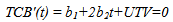 | (3) |
so that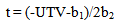 | (4) |
From Eq. (2), the slope of the price-time curve at construction duration determined in Eq. (4) is  | (5) |
By referring to Eq. (1), the bid price equation can be given by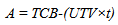 | (6) |
From Eq. (6), the slope of the TCB Iso-Line can be obtained as | (7) |
From Eq. (5) and Eq. (7) it is concluded that the slope of the price-time curve at the duration that minimizes TCB is equal to the slope of the TCB Iso-Line. Therefore, the TCB Iso-Line that is tangent to the price-time curve of the contractor determines the most competitive strategy (see Figure 2).
3. Data Preparation
The data used in this study are obtained from the Oklahoma Department of Transportation (ODOT). The dataset consists of all the completed price-time bi-parameter bidding projects that ODOT has let. Contractors that had three or more A+B projects with ODOT are selected for further analysis in this study due to the minimum number of data points required in developing a price-time curve. The historical database contains 54 data points for 14 contractors. The summary of the data is provided in Appendix.The completed A+B projects have different budgeted costs and durations. For instance, contractor K completed four A+B projects that are different in terms of award bid, final construction price, final contract time, and days used. In order to develop a contractor’s price-time curve for A+B projects using the bid price and time data of previous A+B projects, the scope free time and price measures are necessary because every previous project’s scope is different. Therefore two indices are developed to represent the cost and time performance of completed A+B projects: Price Index and Time Index. The equations utilized to calculate price and time indices are shown in Eq. (8) and Eq. (9): | (8) |
 | (9) |
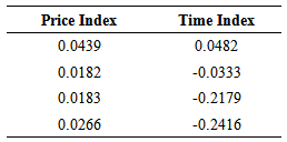
Price index is measured by dividing the amount of price over-runs by the award bid price. If the final construction price of a project is less than the award bid, it means that the contractor has been able to save in construction costs, which results in negative price index. A positive price index, on the other hand, is an indicator of construction cost over-runs. A zero price index means the project’s final construction price has been equal to award bid. Time index is measured by dividing the number of days that a project is finished late by the final contract time. A negative time index indicates time savings, which makes the contractor eligible for monetary incentives while a positive time index is an indicator of schedule overruns, which results in disincentive payments to the contractor. A zero time index means the project’s duration has been the same as contract time. Values of price and time indices that are less than zero indicate good project performance, whereas values of time and price indices that are greater than zero indicate poor project performance. Table 1 shows the time and price indices for Contractor K. The first row of this table indicates a project that has both cost and schedule overruns. This project was awarded for $4,078,000, but after completion of project the final construction price was $4,257,000, resulting in price index of 4.39%. In addition, the final contract time of this project was 166 days while the final project duration or days used was 174 days, resulting in a time index of 4.82%. The time and price indices are calculated for all projects. Then the analysis of variance (ANOVA) is performed to investigate the relationship between price and time indices.Table 1. Time and Price Indices for Contractor K
 |
| |
|
4. Development of Price-Time Relationship Models
The entire analysis process is explained using the contractor K’s data. Figure 3 shows the entire procedure of developing price-time relationship model for this contractor. After calculating the price and time indices of completed A+B projects, the price index is fit to linear and quadratic functions of time index. The ANOVA and regression analyses are performed for linear and polynomial functions separately. Then the R-squared and P values of the linear and polynomial models are compared and the best model is selected.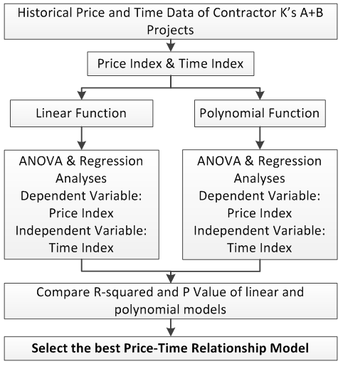 | Figure 3. The Procedure Used to Develop Price-Time Relationship Models |
5. Regression Results
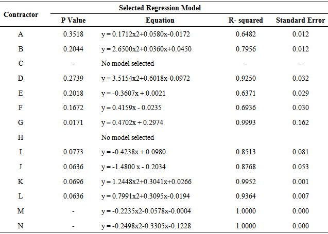
The ANOVA and regression analysis is performed for all the contractors individually. The results of the analysis are shown in Table 2. For each contractor the ANOVA reveals whether or not the relationships between the dependent and independent variables (Price Index and Time index respectively) are significant. The regression analysis also results in linear and quadratic equations that relate price index to time index combined with the R-squared values, which is a goodness of fit factor.Table 2. Results of ANOVA and Regression Analyses for ODOT Contractors
 |
| |
|
A quadratic regression model performs better for contractors A, B, D, K, L, M, and N. A linear regression model outperforms the quadratic model for contractors E, F, G, I, and J. The regression models are selected based on their P-value as well as R-squared value. A model with a lower P value better explains the variability of the independent variable. If the P values of linear and polynomial regression models are equal, the model with larger R-squared value is selected. Neither linear regression nor polynomial regression is significant for contractors C and H.
6. Price-Time Curves
In the previous section, the significant regression equations that best explain the relationship between price index and time index for different contractors were identified. Except for contractors C and H that neither linear nor quadratic equations are significant, the price-time curves are developed for other contractors. The process of developing price-time curves from the regression equation is explained for contractor K. The same calculation process is applied to other contractors as well. After replacing y with price index and x with time index the fitted model for contractor K is: Where A = final construction price; D = days used; A0 = award bid; and D0 = final contract time.By rearranging the equation we will have the following equation:
 | (10) |
This equation illustrates the internal relationship between the bid price and time for contractor K. The functional relationship between bid price and time is determined by deciding (D0, A0). The (D0, A0) can be the SHA’s or contractors’ estimate about the expected duration and price of the project at the normal point. The normal point is the location on the price-time curve where the construction cost is the minimum.
7. Application of Price-Time Models
One project is selected to demonstrate how a price-time model can be successfully applied to determine the optimum UTV and I/D rates that maximizes the competition during the bid process. The selected project contract number is 050639 with the bid days of 365 and award bid of $18,464,000. The duration of 365 days is the maximum allowable construction time defined by the owner prior to letting the project. Contractor L won the A+B bid competition in this project. The competitiveness of contractor L is compared with other contractors under different UTVs in order to study how UTV impacts the competitiveness of contractors during the bid process.Assume that five contractors (D, J, L, B and K) are participating in the bid process. These contractors have the most significant price-time curves in terms of R-squared and P value. In addition, the contractors have a high number of completed A+B projects (either four or five projects). The price-time curves of these five contractors are illustrated in Figure 4. The area above the bold face line in Figure 4 shows the bid strategies that are noncompetitive for any UTV. The bold face line represents the bidding strategies that have a chance of winning the contract. This competitive line that represents the most competitive strategies in the bid process is made of the price-time curves of contractors D, J, and L. In other words, the entire bidding strategies of the other contractors (B and K) are noncompetitive for any UTV. The competitiveness of contractors is evaluated for different UTVs in order to identify the UTV intervals that make each contractor competitive in the bid process.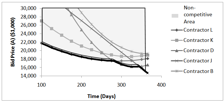 | Figure 4. Price-Time Curves of Contractors |
Three scenarios are designed to investigate the competitiveness of contractors D, J, and L during A+B bid process. In the first scenario, the UTV is assumed to be equal to zero, meaning that there would be no monetary incentives for early completion. The second scenario investigates a situation where the UTV is equal to $25,000/day. The third scenario is a situation when the UTV is equal to $35,000/day.
7.1. Scenario I
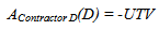
In the first scenario the UTV is assumed to be zero, thus in this bid process there would be neither incentive for early completion nor disincentive for late completion. This scenario is illustrated in Figure 5 where slopes of TCB Iso-Lines are equal to zero. The most competitive strategy of each contractor is the point where a TCB Iso-Line with the slope of zero is tangent to the price-time curve of contractors. Since the price-time relationship for contractor J is linear, the most competitive strategy for this contractor would be the point where TCB Iso-Line passes through the point with the lowest bid price, which occurs at the maximum allowable contract time (365 days). In this scenario, contractor J would be the most competitive contractor due to its ability in proposing the lowest bid price among competing contractors.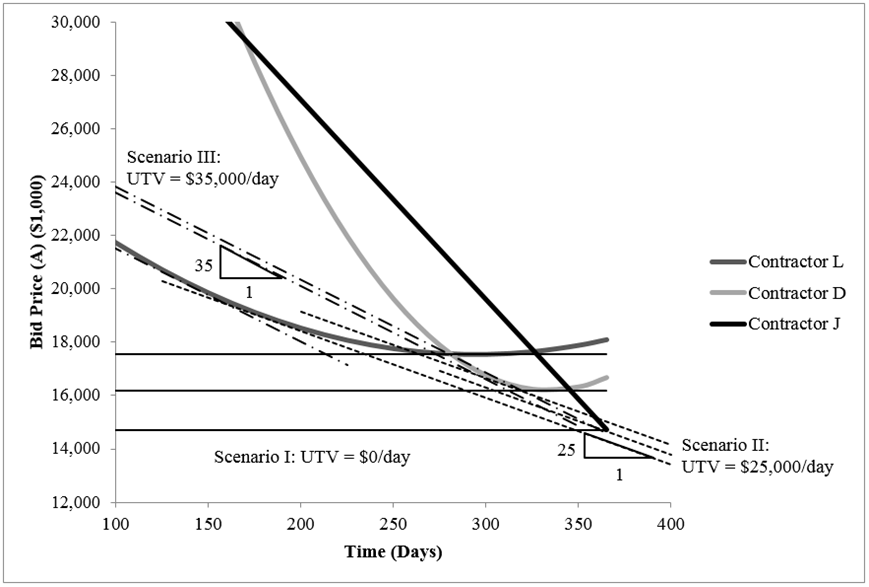 | Figure 5. Three Case Scenarios |
The total combined bid is calculated for these three contractors when UTV is equal to zero dollars per day. For contractors D and L, the most competitive strategies are the points on their price-time curves where the slope is equal to zero. The most competitive strategies of contractors D and L when UTV is equal to zero are calculated as below: | (11) |
 | (12) |
so that-325.2132+0.9744 D = 0By solving for D, the most competitive duration for contractor D is 334 days. By inserting this duration in Eq. (13), the most competitive bid price for contractor D is $16,193.74. | (13) |
 | (14) |
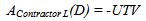
so that-65.191+0.2214D = 0Solving for D, the most competitive duration for contractor L is 295 days. By inserting this duration in Eq. (15), the most competitive bid price for contractor L is $17,548.059.For contractor J, however, the most competitive strategy is the lowest bid price point, which can be calculated by inserting the maximum allowable contract time (365 days) in Eq. (17). 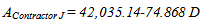 | (15) |
The most competitive bid price at 365 days is equal to $14,708.42.
7.2. Scenario II
In Scenario II, the UTV is equal to $25,000/day, thus in this bid process contractors are paid $25,000/day incentives for early completion of project or charged the same amount for late completion. This scenario is illustrated in Figure 5 where slopes of TCB Iso-Lines are equal to -25. The most competitive strategy of each contractor is the point where a TCB Iso-Line with the slope of -25 is tangent to the price-time curve of contractors. Since the price-time relationship for contractor J is linear, the most competitive strategy for this contractor would be the point where TCB Iso-Line passes through the point with the lowest bid price, which occurs at the maximum allowable contract time (365 days). In this scenario, contractor L would be the most competitive contractor due to its ability in proposing the lowest TCB among competing contractors.The total combined bid is calculated for these three contractors when UTV is equal to $25,000/day. For contractors D and L, the most competitive strategies are the points on their price-time curves where the slope is equal to -25. The most competitive strategies of contractors D and L when UTV is equal to 25 are calculated as below: By inserting UTV in Eq. (14) the following equation is obtained:-325.2132+0.9744 D = -25By solving for D, the most competitive duration for contractor D is 308 days. By inserting this duration in Eq. (13), the most competitive bid price for contractor D is $16,514.44.By inserting UTV in Eq. (16) the following equation is obtained: -65.191+0.2214D = -25Solving for D, the most competitive duration for contractor L is 182 days. By inserting this duration in Eq. (15), the most competitive bid price for contractor L is $18,959.54.For contractor J, however, the most competitive strategy is the lowest bid price point, which can be calculated by inserting the maximum allowable contract time (365 days) in Eq. (17). The most competitive bid price at 365 days is equal to $14,708.42.
7.3. Scenario III
In Scenario III, the UTV is equal to $35,000/day, thus in this bid process contractors are paid $35,000/day incentives for early completion of project or charged $35,000/day disincentive for late completion of project. This scenario is illustrated in Figure 5 where slopes of TCB Iso-Lines are equal to -35. The most competitive strategy of each contractor is the point where a TCB Iso-Line with the slope of -35 is tangent to the price-time curve of contractors. Since the price-time relationship for contractor J is linear, the most competitive strategy for this contractor would be the point where TCB Iso-Line passes through the point with the lowest bid price, which occurs at the maximum allowable contract time (365 days). In this scenario, contractor L would be the most competitive contractor due to its ability in proposing the lowest TCB among competing contractors.The total combined bid is calculated for these three contractors when UTV is equal to $35,000/day. For contractors D and L, the most competitive strategies are the points on their price-time curves where the slope is equal to -35. The most competitive strategies of contractors D and L when UTV is equal to 35 are calculated as below: By inserting UTV in Eq. (14) the following equation is obtained:-325.2132+0.9744 D = -35By solving for D, the most competitive duration for contractor D is 298 days. By inserting this duration in Eq. (13), the most competitive bid price for contractor D is $16,822.335.By inserting UTV in Eq. (16) the following equation is obtained: -65.191+0.2214D=-35Solving for D, the most competitive duration for contractor L is 136 days. By inserting this duration in Eq. (15), the most competitive bid price for contractor L is $20,314.545.For contractor J, however, the most competitive strategy is the lowest bid price point, which can be calculated by inserting the maximum allowable contract time (365 days) in Eq. (17). The most competitive bid price at 365 days is equal to $14,708.420.
8. Summary
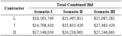
The analysis of these three scenarios clearly indicates that the UTV selected by the owner can change the competitiveness of contractors participating in the A+B bidding process. Table 3 shows total combined bid comparison of contractors for the three scenarios. Since unit price in the equations is equal to $1,000, the total combined bids in this table have been multiplied by 1,000 to represent the real prices. When the UTV is equal to zero and contractors do not receive incentives for early completion, contractor J is the most competitive contractor with the following relationship: TCB(J) < TCB(D) < TCB(L). In the second scenario where the UTV is equal to $25,000/day, contractor L becomes the most competitive contractor and the following relationship is obtained: TCB(L) < TCB(J) < TCB(D). And in the third scenario where UTV is equal to $35,000/day contractor L remains the most competitive contractor followed by contractor D and contractor J. Thus the following relationship holds in the third scenario: TCB(L) < TCB(D) < TCB(J).Table 3. Total Combined Bid Comparison of Contractors for the Three Scenarios
 |
| |
|
By gradually increasing UTV from zero, different situations are created in terms of the competitiveness of contractors. These UTVs are determined and named as thresholds in this study. The first situation created after increasing UTV from zero is where the competitiveness of contractor D and contractor L becomes equal. The slope of TCB Iso-Line that is tangent to the price-time curves of contractor D and contractor L is equal to -18.805 meaning that the UTV that equalizes the competitiveness of these contractors is $18,805/day. The second UTV threshold is where the competitiveness of contractor J and contractor L is equal. In this situation the UTV is equal to $23,128/day and both contractor J and contractor L have the most competitive strategy. And finally, by increasing the UTV to $31,366 a situation is developed where the competitiveness of contractor J and contractor D are equal. Figure 6 shows the winning situations for this case analysis. Based on different UTVs and the price-time curves of contractors, two winning situations can be identified in this A+B bid competition. The line that passes through contractor J’s price-time line and is tangent to the price-time curve of contractor L is where both contractors have the same level of competitiveness which happens when the slope of the TCB Iso-Line is equal to -23.128 or the UTV is equal to $23,128/day. Region “a” indicates the situation where contractor L has the most competitive strategy. For any UTV greater than $23,128/day or for any steeper TCB Iso-Line, contractor L would be the most competitive contractor. Region “b” is the winning situation for contractor J. Any UTV less than $23,128/day or any shallower TCB Iso-Line makes contractor J the most competitive contractor.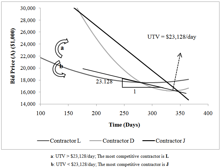 | Figure 6. Winning Situations vs. UTV |
According to the historical data, the real UTV for this project was $4,500/day, which falls into region “b”. Contractor J is the most competitive contractor in this situation. However, in the actual A+B bidding process, contractor J did not participate. The results of this study suggest that if contractor J had participated in the bid process, this contractor would had a very high possibility to win this project.There are also significant implications in the findings of this study for the owner’s practice in implementing an A+B contracting method. Usually the project owner has two goals in using an A+B bidding method: 1) to encourage contractors to compete over the original bid price (A), and 2) to compete with each other to propose lower bid days in order to minimize the negative impact on the traveling public. Project owners should realize the full impact of selecting the UTV for bidding projects. If the UTV is very low, only contractors that are able to propose the lowest bid price will likely have a chance to win the project and those that are capable of accelerating construction are not competitive. If the UTV is very large, contractors that are capable of reducing the project duration are very likely to win the competition; whereas, those that can reduce the bid prices, but not the duration, are less competitive. In addition, contractors may adjust their bid proposal and propose a lower price and/or duration, if their most competitive strategy is very close to other contractors’ competitive strategies and they are convinced that they are likely to win if they slightly change their strategies. When the vast majority of contractors are strictly noncompetitive, contractors are discouraged to propose lower bid prices and/or durations.The actual UTV that ODOT used for project #050639 is $4,500/day. This UTV creates a situation where contractor J would become the most competitive contractor during the bid process. However, this value is not high enough to stimulate competition between contractors because contractor L and contractor D are far from having the most competitive strategy. In addition, this encourages contractor J not to offer its most competitive strategy by knowing that they are by far the most competitive contractor in the competition. The actual UTV used in this project does not encourage contractors to propose accelerated bids.
9. New Formula Measuring Level of Competition
As shown in the results of the case study, when UTV is equal to zero, the total combined bid of contractor J is $1,485,320 less than contractor D and $2,839,639 less than contractor L. When UTV is equal to $18,805/day, the total combined bid of contractor J is $714,262 less than contractors D and L. When UTV is equal to $23,128/day, the total combined bid of both contractors J and L are only $487,800 less than contractor D. For an UTV of $31,366/day the difference between the total combined bid of contractor L and contractors D and J is $1,588,124. In other words, in some situations the competitive strategies of contractors are closer to each other, which create a situation that stimulates contractors to propose accelerated construction durations. A new formula can be developed in order to measure the level of competition in an A+B bidding project. This formula measures the average of differences between contractors’ total combined bids. A lower average of differences between contractors’ TCBs indicates a higher level of competition between contractors. This formula can be used by SHAs to maximize the competition during bid process. The following is suggested as a measurement: | (16) |
Where TCB = Total Combined Bid; n = number of contractors that have a chance to win; and i ={1,…,n}. This new value has been calculated for the contractors in the case study when UTV is equal to $0/day, $18,805/day, $23,128/day, and $31,366/day (Figure 7). The average difference between contractors’ TCB is equal to $1,893,093 when the UTV is equal to zero. When the UTV is equal to $18,805/day the average difference between contractors’ TCB is equal to $714,262. When the UTV is equal to $23,128/day the average difference between contractors’ TCB is equal to $487,800. And finally, when the UTV is equal to $31,366/day, the average differences between contractors’ TCB is equal to $1,588,669. It can be clearly seen that the average of difference between contractors’ TCB is the lowest when UTV is equal to $23,128/day. If contractor D proposes a TCB that is $487,800 lower than their ideal TCB, their chance of winning the competition increases significantly. In addition, contractors L and J, which have the same level of competitiveness, are also required to propose a lower TCB than their ideal strategy in order to remain competitive. In this situation, all the contractors know their competitors can potentially be the winner and do their best to propose a price and duration that cannot be easily dominated by others. Therefore, $23,128/day would be the UTV that maximizes competition between contractors.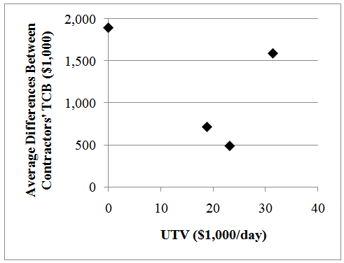 | Figure 7. Level of Competition for Different UTVs |
10. Limitations
There are some limitations in this study. It has been assumed that for each contractor there is only one price-time for any type of A+B projects. Most A+B projects are urban highway rehabilitation projects but, a project’s level of scale, complexity, location and other factors may affect the price time curve. However, due to limited number of completed A+B projects in Oklahoma, this study assumed one price-time relationship without considering the possible effects of external project characteristics. Developing multiple price-time models based on different A+B project types would be a reasonable extension to this study.
11. Conclusions
This paper evaluated the impacts of UTV on the competitiveness of contractors in A+B bidding projects. The results of ANOVA and regression analysis indicated that for the majority of contractors there is a significant relationship between time and bid price. The price-time models for contractors of ODOT were developed utilizing the historical A+B bidding data. The three scenario analyses clearly demonstrated how different UTVs change the level of competition in A+B bidding and may result in different winning contractors. The results suggested that the conventional approach that only takes road user costs into account in order to determine the UTV and incentive/disincentive rates for A+B bidding projects might result in sub-optimal results. A new formula was developed to calculate the average of differences between contractors’ TCB. By testing different UTVs with this formula, the owner can determine and adjust the UTV to ensure a stimulated competition during the bid process. This study laid a computational foundation that enables State Highway Agencies (SHAs) to determine the optimum UTV and I/D rate that maximize the competition among contractors and result in selection of the most efficient contractor in construction acceleration. It also introduces an approach for contractors to study the strategies of their competitors before proposing a bid price utilizing the publically available bid data.
ACKNOWLEDGEMENTS
The authors would like to thank Mr. Gary Evans, chief engineer, Mr. George Raymond, State Construction Engineer, and Ann Wilson from the Oklahoma Department of Transportation, for sharing their knowledge and experience during the course of this research and also providing the historical A+B bidding data. This research was funded by the Oklahoma Transportation Center.
References
| [1] | American Society of Civil Engineers (ASCE) (2013), 2013 Report Card for America’s Infrastructure, <www.infrastructurereportcard.org>. |
| [2] | Moussourakis, J., and Haksever, C. (2010). "Project Compression with Nonlinear Cost Functions." J. Constr. Eng. and Manage., ASCE, 136(2), 251-259. |
| [3] | Falk, J. E., and Horowitz, J. L. (1972). "Critical Path Problems with Concave Cost-Time Curves." Management Science, 19(4), 446-455. |
| [4] | Fick, G., Cackler, E. T., Trost, S., and Vanzler, L. (2010). "Time-Related Incentive and Disincentive Provisions in Highway Construction Contracts." Transportation Research Board, National Research Council, National Cooperative Highway Research Program (NCHRP) Report 652, Washington, D.C. |
| [5] | Herbsman, Z., and Ellis, R. (1992). "Multiparameter Bidding System - Innovation in Contract Administration." J. Constr. Eng. and Manage., ASCE, 118(1), 142-150. |
| [6] | Herbsman, Z. J., Chen, W. T., and Epstein, W. C. (1995). “Time Is Money: Innovative Contracting Methods in Highway Construction,” J. Constr. Eng. and Manage., ASCE, 121(3), 273-281. |
| [7] | Anderson, S., and Damnjanovic, I. (2008). "Selection and Evaluation of Alternative Contracting Methods to Accelerate Project Completion." Transportation Research Board, National Research Council, National Cooperative Highway Research Program (NHCRP) Synthesis 379, Washington D.C. |
| [8] | Christiansen, D. L. (1987). "An analysis of the use of incentive/disincentive contracting provisions for early project completion." Proc., National Conference on Corridor Traffic Management for Major Highway, Transportation Research Board, Washington, D.C., 69-79. |
| [9] | Jaraiedi, M., Plummer, R. W., and Aber, M. S. (1995). "Incentive/Disincentive Guidelines for Highway Construction Contracts." J. Constr. Eng. and Manage., ASCE, 121(1), 112-120. |
| [10] | California Department of Transportation (Caltrans) (2000). "Delegation of Authority for Use of A+B Bidding and Incentive/Disincentive (I/D) Provisions." Memorandum, <http://www.dot.ca .gov/hq/oppd/design/m061200.pdf> (Nov. 7, 2012). |
| [11] | Federal Highway Administration (FHWA) (1989). "Technical Advisory: Incentive/Disincentive (I/D) for Early Completion." Technical Advisory: I/D for Early Completion, <http://www.fhwa .dot.gov/construction/contracts/t508010.cfm>(Nov. 7, 2012). |
| [12] | Arditi, D., Khisty, C. J., and Yasamis, F. (1997). “Incentive / Disincentive Provisions in Highway Contracts.” J. Constr. Eng. and Manage., ASCE, 123(3), 302-307. |
| [13] | Shr, J.-F., Ran, B., and Sung, C. W. (2004). "Method to Determine Minimum Contract Bid for A + B + I /D Highway Projects." J. Constr. Eng. and Manage., ASCE, 130(4), 509-516. |
| [14] | Shen, L., Drew, D., and Zhang, Z. (1999). “Optimal Bid Model for Price-Time Biparameter Construction Contracts.” J. Constr. Eng. and Manage., ASCE, 125(3), 204-209. |
| [15] | Shr, J., and Chen, W. (2004). "Setting Maximum Incentive for Incentive/Disincentive Contracts for Highway Projects." J. Constr. Eng. and Manage., ASCE, 130(1), 84-93. |
| [16] | Callahan, M. T., Quackenbush, D. G., and Rowings, J. (1992). Construction project scheduling, McGraw-Hill, New York. |
| [17] | Shr, J. F., and Chen, W. T. (2003). "A method to determine minimum contract bids for incentive highway projects." International Journal of Project Management, 21(8), 601-615. |
| [18] | Wu, M.-L., and Lo, H.-P. (2009). “Optimal Strategy Modeling for Price-Time Biparameter Construction Bidding.” J. Constr. Eng. and Manage., ASCE, 135(4), 298-306. |

 Abstract
 Reference
 Full-Text PDF
 Full-text HTML