1. Introduction

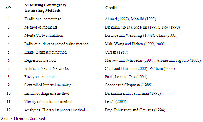
The construction industry is faced with the frequently asked industrial questions of; “why contingency in virtually every form of project execution even in domestic budgeting”? The response usually is that any project yet undertaken has a certain degree of risk which gives rise to the controversy of risk absorption and contingency cost application. It is important therefore to interface both concepts like a typical physical system of forces with the attendant aim of resolving them for a resultant effect. There seems to be a chronological inquiry into this subject particularly by Association for the Advancement of Cost Engineering (AACE, 2009) on project scope development processes and definition, Baccarini (2006) on the concept of estimating project cost contingency, Hollmann (2009) on Monte-Carlo challenge to risk simulation by parametric evaluation. This was an appendage to the original work of Hackney (1997), Merrow, Kenneth and Christopher (1991) and Trost and Garold (2003). Their research response, midwifed the development of empirically-based parametric models that showed how poor scope definition resulted in greater cost and wider project cost accuracy ranges.

However, contingency cost estimation is well researched in construction projects literatures, but how and why the contingency amount considering the risk elements it responds to, is computed and arrived at remains empirically subjective. This paper reviewed the various methods of computing contingency cost and proposed a forward difference summation by an orthogonal function method. The need to set aside a certain sum of money to offset risk impacted items (cost and time wise) resulted in construction industry’s policy of contingency fund (Mak and Picken 2000 and Leach, 2003). How representative and precise the contingency estimating methods are remains a subject of controversy in the construction industry (Curran, 1989, Oberlander and Trost, 2001 and Rad, 2002). However, several methods and approaches to contingency cost estimation have been offered by academics in the industry, yet the unseeming aspect of indeterminacy and subjectivity remains irresolute. The quest for a non bias, non subjective and representative method of estimating contingency have led to the derivation of generic sophisticated techniques with scientific credence. Much of these approaches is found in the works of Pack, Lee and Ock (1994), Chen and Hartman (2000), Clark (2001) and Baccarini (2006). However, neither of these methods offers a concise and representative, yet distributive way of estimating contingency sum on the basis of the various construction work items considering, continuing their risk cost components. This paper asserts that each item of work with their unit rate cost value should contribute dynamically their intrinsic risk cost components to contingency cost.

2. An Overview of Risk and Contingency in Construction Project

AACE (2012) reported that any amount added to an estimate to allow for conditions or events for which the state, occurrence, or effect is uncertain and that experience shows will likely result, in aggregate or an additional cost is regarded as contingency. Views on this subject are diverse in the sense of application and computation. Hence, identification of its characteristics were enumerated by Baccarini (2008) as tolerance in specification, float in schedule and money in the budget. The volatile nature of contingency made Patrascu (1998) to aver that there is no standard definition for contingency and its management and use is limited to the end-user. Because of its time effect on schedule, PMI (2000) recognized it as the amount of money or time needed above the cost estimate to reduce the risk of overruns of project objectives to a level acceptable to the organisation. Clark and Lorenzoni (1985) stated that allowance is the cost for specific, known but undefined items. This was also the views of Patrascu (1998), Querns (1989) and Rad (2002). In a slow contrast, management reserve has been viewed as a provision (provisional cost) held by the client for possible changes in project scope and quality (Widerman, 1992). The radius of coverage of management reserve was narrowed by Yeo (1990) to include but not limited to extra ordinary, unforeseen eternal risks, like currency-exchange fluctuation rate, force majeure, etc.

Abdou, Lewis and Alzarooni (2007) comparatively noted that all project types involve risks of various kinds and types. Flanagan and Norman (1993) had earlier stated that the construction industry is infested with more risk than other industries. Consequently, Abdou et al. (ibid) emphasized that in construction projects, risk and uncertainties are of several types. Limited lists of risk types were listed to include political, financial, economical, environmental and technical. It was reported that many of these uncertainties will ultimately impact on the financial status negatively or positively than anticipated. In view of the inherent and apparent effect of slow response to risk diffusion in construction projects, Flanagan and Norman (1993) averred that the industry has been a little faster than snail speed in responding to risk impacts and slow realization to the potential benefits of risk management. Chapman and Curtis (1991) and Abdou et al (2007) identified the reason for this slow response to risk analysis and management in the industry to include organizational culture, negative attitudes and mistrust of risk analyses methods as the main reasons behind the prevention of its use. Hollman (2007) and AACE (2009) identified the various risk types and categorized them into two. This paper intends to respond to risks that have predictable relationships to overall project cost growth which are dispersed with contingency cost. Hollmann (2007) labeled these classes of risk as “systemic” and “project specific” risks. Systemic risk has been identified to be the soul of the project “systemic” risk, culture, business strategy, process system complexity, technology etc. Hackney (1997) showed that the impact of some of these risks are measurable and to a large extent predictable between projects within a system and to some extent within the industry as a whole. Estimation of these risks have been generally acknowledged to be known even at cost planning stage (AACE, 2009). This is the basis on which tolerable values are given to cost of items in a Bill of Quantity to accommodate the unforeseen circumstances.

3. What Constitutes Contingency

From existing literatures, we have been able to identify the following response attributes of contingency cost application to include management reserve to rescue cost risk (PMI 2000), Risk and uncertainty in a project (Thompson and Perry 1992), unforeseen events defined within the project scope (Moselhi 1997, Yeo 1990), unknown site conditions (PMI 2000), unexpected events (Mark et al 1998), unidentified events in the course of construction (Levine 1985) or undefined items and scope of labour (Clark and Lorenzoni and Thompson and Perry 1992). Further, Baccarini (2008) noted some features of contingency to include risk management strategies such as risk transfer, risk reduction and financial treatment for retained risk by application of contingency. These attributes showed a blend of risk treatment strategies in conjunction with contingency as a total commitment feature by using contingency cost to avoid the need to appropriate additional funds and reducing the impact of overrunning the cost objective.

Contingency usually excludes major scope changes, such as changes in end product specification, capacities, building sizes and location of the project. It also excludes extraordinary events such as major strikes and natural disasters, management reserves and escalation effects. Some of the items, conditions, or events for which the state, occurrence and/or effect is uncertain include, but are not limited to planning and estimating errors and omissions, minor price fluctuations (other than general escalation), design developments and changes within the scope, and variations in market and environmental conditions.

This paper identifies the possible risks of project specific and systemic risk to be associated with construction projects. AACE (2009) had highlighted typical project specific risks and systemic risks to include Basic Design, level of technology, process complexity, material impurities at project definition stage I, and at stage II to be site/soil requirements, engineering and Design, health, safety, security, environmental planning and schedule development. Stage III, include estimate inclusiveness, team experience / competency, cost information available and estimate bias. These three (3) phases are peculiar to systemic risks. Flyvbjerg (2006) had proposed the reference class forecasting method as a means of their estimate validation. On the other hand project specific risks have on the basis of estimate classification, include but not limited to weather, site subsurface conditions, delivery delays, constructability, resource availability, project team issue, quality issues etc. This breakdown of risk types explains why an interaction of risk weight/factor into contingency estimating is interfaced for optimal understanding and quantification

4. Risk and Contingency Estimating Methods

The construction industry is in dare need of an estimating framework that seems to interface the estimation of contingency, cost and risk value, in interface to a specific project. AACE (2008) had suggested that any method developed for this purpose should be able to address the following foundational principles;

● Meeting clients objectives, expectations and requirements

● Facilitating effective decision or risk management process.

● Fit-for-use

● Identifying the risk drivers with input from all appropriate entities

● Clearly link drivers and cost/schedule outcomes.

● Avoiding iatrogenic (self-inflicted) risks

● Employing empiricism

● Employing experience/competency

● Providing probabilistic estimating results in a way that supports effective decision making and

● Risk management.

Fortunately most of the methods before now for estimating risks and contingency seems to address some of these issues in their empirical forms as evident in the works of Flanagan and Norman (1993), Raftery (1994), Byrne (1996), Grey (1998), Smith (1999) PMI (2000). These methods addressed the problems of risk premium, Risk – adjusted Discount Rate, subjective probability; Decision Analysis; Sensitivity Analysis, Expected Monetary Value (ENPV); Monte Carlo Simulation; Portfolio Theory and Stochastic Dominance and the application based softwares such as Casper @ Risk or CrystaBall, techniques.

Table 1. Summary of Contingency Cost Estimating Methods

Baccarini (2006) also reported a range of contingency estimating techniques that tends to address overrunning impact on project cost. Literatures that reported these techniques includes, Traditional Percentage method, (Ahmad, 1992 Moselhi 1997), Method of moments (Dickmann 1983, Moselhi 1997, and Yeo 1990), Monte Carlo Simulation method, (Lorance and Wendling 1999, Clark 2001) individual risks – expected value method (Mak, Wong and Picken 1999, 2000), Range Estimating method (Curran 1987), Regression method, (Merrow and Schroeder 1991, Aibinu and Jagboro 2002), Artificial Neural Networks, (Chen and Hartman 2000; William 2003), Fuzzy sets (Paek, Lee and Ock, 1994), controlled interval memory (Cooper and Chapman 1985), influence Diagrams method, (Dickmann and Featherman 1998), theory of constraints method (Leach 2003) and Analytical Hierarchy Process method (Dey, Tabucanon and Ogunlana 1994). Unfortunately, none of the methods on either sides of Risk and Contingency tend to address the interface between the two as a way of showing the proportioned impact of risk on contingency computation on the basis of probabilistic tendencies i.e. extremes of cost itself.

5. Formative Basis of Theory

Geometrically, all the possible existing intervals in a space are defined by: been b – a interval class, so that a dimensionless space has an infinite interval x < a or x < b that reduces to ∞, when a = b. A space has no length if a ≤ x ≤ b, and reduces itself to a point because of its’ dimensionless property and taken to be the limiting value of a line (Meschenmoser and Shaskkin, 2013, and Gorodestskii, 2006).

If a bill of quantity item of work is considered as a function of cost having a length of L as the cost of the item, then if I₁, I₂, … … … I_n are the interval that exist on the locus of the geometry (been probable costs) which are mutually disjointed than L (I₁ U I₂ U … … U I_n) = L (I₁) + L (I₂) + … … … + L(I_n) such that if the cost () of an item is zero (0), then no interval exist, hence L () = 0 suggesting that the cost of an item is zero (0) when the space is empty. Therefore, the length of an open space been the cost of an item is given by: where I_k is the open/probable intervals (Baushey, 2006 and Chuprunov, 2006). 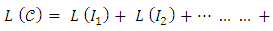It follows that the length If intervals of the cost function are nested into I = [a, b], with a, b been the coordinate value of the items risks components of cost and time, then L () = L (I₁) + L (I₂) + … … … can converge as a pure non-negative number of a closed space existing in [a, b] (Chentsov, 2006). So the available space (range) of a closed space becomes S_c [a, b] which is L (S_c) = b – a – L (S_c) where Sc is the complement in [a, b] of an uncovergible space such that the measure of the space or the range value is greater than zero (0) i.e. m(s) > 0. If the space is properly nested, it follows that the space or range existing under the cost item with all its weight function can be a finite additivity. Suppose and provided S_k are the existing intervals of the space then 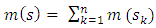is a denumerable additivity arising from the variability nature of the range value or space. The monotonictic properties also holds for the space as S₁ S₂ when m(S₁) < m (S₂). As a parallel, an item of a Bill of Quantities is idealized as (S) truncated in the interval of [a, b], the measure of the space (S) is elated by m(S) = b – a – M_e(S`). The interior measure of the space M(S) shows semblance with the least upper bound of a length of a close space (S_c) contained in (S) i.e. m_i(s) = l.u.b.L(Si). This space becomes measurable when the interior measure is equal to the exterior measure i.e. m_i(s) = M_e(S) and M_i (S) < M_e(S). If the space is thought of as a partial sum of a truncated spaces, S₁ and S₂ which are distinctively disjointed spaces then, m(S₁ S₂) = m(S₁) + m(S₂). When the exterior value of (S) is zero i.e. m(S) = 0. Moreso, S₁ S₂ when m(S₁) < m(S₂). With a countable measure, S₂ – S₁ is valuable so that m(S₂ – S₁) = m (S₂) – m(S₁). When all partial spaces obeys S₁ S₂ S₃ … … … ,then . This becomes measurable by 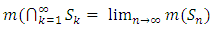which is also true for and also measurable by

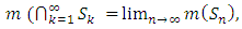
Supposedly, unit rate of cost items in a bid of bill of quantity are derived as optimistic oscillatory scalar quantity products of cost and time that are statistically adjudge to actualize the construction of a particular item of work. Such statistical permisivity is fraught with probability values generated by the risk weight component of the items that are intrinsically linked to the pessimistic and optimistic spatial reference considered as interval/space that transit to an acceptable value, to be known as item unit cost rate. The space between these extremes portends a probability attribute which are in this study referred to as lower and upper infimium.

6. Orthogonizing Contingency Cost Estimation

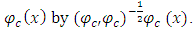
On the basis of Harry Bateman theory of orthogonal function, this paper draws a parallelism approach to conceptualize items in the various elements of a Bill of Quantities as a summable value that constitutes an orthogonal entity for which all elements and their item rate constitute a system of orthogonal function. 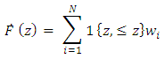Then if is a weight function of determinate risk component of contingency cost and time of a project, then is the tolerable value or permissible value given to an item to show the limiting influence on other items in a weighted mean operation. The application of information theoretics suggests the attachments of weights to observations of interest to reflect an estimate of data-generating distribution (Nevo, 2002). Such weight response measure minimizes the distance between empirical and estimated distribution (Imbens, 1997, Imbens, Spady and Johnson, 1998, Hellerstein and Imbens, 1999 and Qin and Lawless, 1994). Normalization of distribution to enable precise estimation of data by the attachment of weight or probability factors (e.g. risk) elements is well rehearsed by Imbens (1993, 1997) and Nevo (2002) using indicator function as 1{.}. Subjecting observed data to equal weight of certain value conforms the distribution to empiricism (Nevo, 2002) such that the corresponding estimate of the weighted distribution becomes;

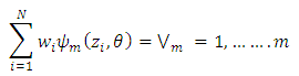
Provided such moments of all the weighted sample analog vanishes, reminiscent of an orthogonal scalar products. Nevo (2002) showed this to be;

Relatively, the entire unit rate cost of work items in a Bill of Quantity are considered as a set of distribution

having risk probability components that may impact their normality on schedule without deviation. Consequently, estimating their normalization requires the introduction of weights attached to their original parameter of interests.

The risk weight of contingency are the scalar operators; cost and time With a limiting interval of minimum (a) and maximum (β) of the two scalar operators and a weight product of

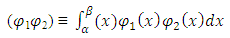(1)

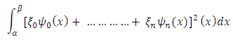
This is defined for all contingency components for which is quadratically integrable in the limiting interval (Kacinskaite and Laurincikas, 2008). In line with stieltjes integral, the cost and time scalar product component of contingency can be generalized as;

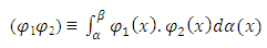(2)

Where been the minimum values of the scalars is a non decreasing function. When experiences a jump by the effect of the weight function of Risk to the point that the project is infested with indeterminacy in terms of its cost and time with magnitude then the scalar product reduces to a sum (Rozovsky, 2010, and Gotze and Zaitsev, 2009);

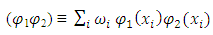(3)

By this summation, contingency is viewed as a discrete variable consisting of work items in Elements of the traditional Bill of Quantities. For the possibility that cost and time risk components can be zero in a project i.e. a steady construction sequence that does not warrant cost and time escalation, then the contingency orthogonal property can be set as;

(4)

So that any other indeterminate component of contingency will form a subset of a linearly independent relation of the form

(5)

remaining invalid in the limiting range , except when forming the scalar product with The variables, forms an orthogonal system, if;

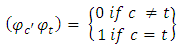(6)

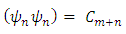
Whereas, every orthogonal system can be normalized by replacing . This forms a finite sequence of linearly independent function of Bill items that is orthogonal with respect to the scalar product of; .

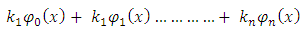
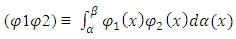By the formation of suitable linear combinations of the Bill items and their attendant risk components such that we may put recurrently

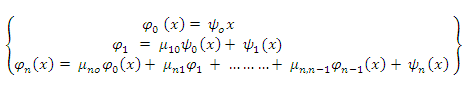(7)

This makes an orthogonal system when

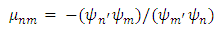(8)

Taking m = 0, 1, … … …, n – 1, a collolary to this, is by putting all the Bill items which constitute risk values and by extension contingency into a system of orthogonal functions as;

(9)

On determination of the risk coefficients from the orthogonal system leads to;

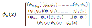(10)

Having established that the Bill items constitute risk components and validly cost and time components of contingency, and further conceptualise that each Bill item formed an orthogonal system of equations in element by element within the interval 0 to n. The orthogonal system in (9) can then be normalize by the introduction of conjugate complex called Gram’s determinant Gn which is the cofactor of in the expression (10) Making . 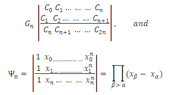Gn the discriminant of the positive definite quadratic form

In , and hence positive with G_-1 = 1. Hence the system of the form (9) is determined uniquely with;

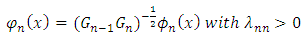(11)

In integral representation form, the determinate can be established as

(12)

If the orthogonal system of the several Bill items constitute several variables then it can be subjected to n-tuple integral over the limiting cost interval for each item and

(13)

We have associated a weight function, ω(χ) as the risk value of a system of orthogonal function on the cost interval of Bill items. Each item in the Bill of Quantities is represented by xⁿ into n-variables, such that the cost arising from the risk constituent can be derived from the moments of the weight function;

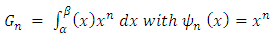(14)

(15)

From Gram’s determinant, we have,

From the result above the contingency of any project can be computed from partial sum of the forward difference of the limiting cost interval of any item in the project Bill of Quantities to a converging summation.

7. Conclusions

Every construction item in a Bill of Quantity has its own risk component in terms of cost and time. The risk weight assigned to any item makes it a proportional factor of variability between two extremes of lower and upper infimium against bid cost rate. The difference between the lower and upper infimium is the oscillatory value that tends to stabilize it to bid cost, beyond which can be used to diffuse the risk cost as contingency. By way of application, all items in bid Bill of Quantity are regarded under the orthogonal function as items of several variables (xⁿ), with their associated rates (cost) are oscillating between the lower infimium (x_∞) and an upper infimium (x_β) representing the pessimistic cost (rate) of the item and the upper infimium representing the optimistic cost. From the proof, we can deduced that a progressive/forward moving partial sum of the difference between the lower and upper infimium been

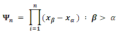Constitutes the project contingency cost. This was kindly made permissible by the associated risk weight function that generated the need for contingency.

ACKNOWLEDGEMENTS

The Authors are indebted of thanks to the copyright holders of the Harry Bateman’s manuscript project whose work formed the basis of this construct.