1. Introduction

A Brain Computer Interface (BCI) is a type of communication system that translates brain activities into electrical commands, enabling the user to control special computer applications or other devices simply by means of his or her thoughts[1, 2]. Such an interface can be used both in neuromuscular disorder clinics and in everyday life. A typical BCI schematic is shown in Figure 1. Brain signals are acquired by electrodes on the scalp and cleaned (i.e., amplified, sampled, and filtered) by preprocessing methods. Once cleaned, their features are extracted and classified to determine the corresponding types of mental activities that the subject performs. The classified signals are then used by an appropriate algorithm for the development of a certain application. Among the various techniques for recording brain signals[1-14], electroencephalography (EEG) is focused in this paper. EEG is most preferred for BCI applications due to its non-invasiveness, cost effectiveness, easy implementation, and superior temporal resolution[1], [9].

Brain signals can be generated through one or more of the following routes: implanted methods, evoked potentials (or event-related potentials), and operant conditioning. Evoked potentials (in short, EPs) are brain potentials that are evoked by the cause of sensory stimuli. Usually they are obtained by averaging a number of brief EEG segments (called EEG trials) corresponding to the stimulus of a simple task. In a BCI application, control commands are generated through the EPs when the subject attempts an appropriate mental task[1],[3],[13-19]. This paper focuses on the EPs recorded at the eight electrodes (Fz, Cz, Pz, Oz, P7, P3, P4, and P8) in Figure 2[3].

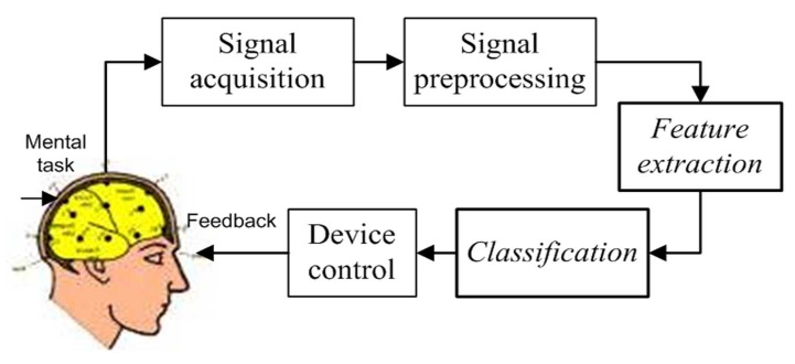Figure 1. Five key steps in BCI (feature extraction and classification are focused)

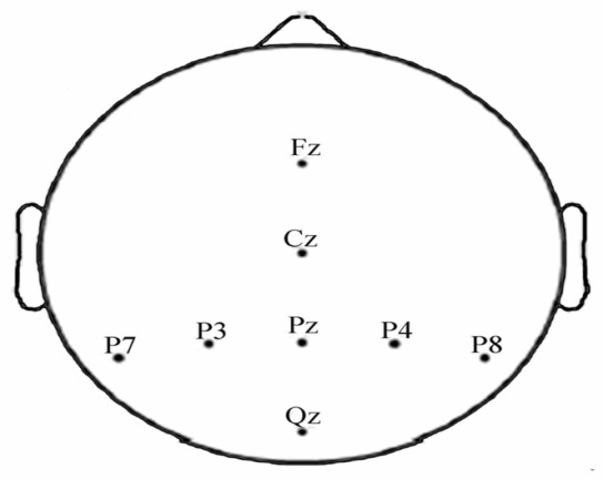Figure 2. Eight electrodes configuration used in experiment

In 1964 and 1965, respectively, Chapman and Bragdon[20] and Sutton et al.[21] independently discovered a wave peaking phenomenon around 300 ms after a task-relevant stimulus. This component is known as the P300. While the P300 is evoked in many different ways, two influencing factors are stimulus frequency (less frequent stimuli produce a larger response) and task relevance. The P300 is fairly stable in locked-in patients and reappears even after severe brain stem injuries[22]. Farwell and Donchin[23] first showed that this signal could be successfully used in a BCI application. Employing a broad cognitive signal like the P300 confers the benefit of control via a variety of modalities enabling discrete control, for example, in response to both auditory and visual stimuli. However, the P300, as a cognitive component, is known to vary with a subject’s fatigue level[3].

Current BCI designs typically incorporate five main steps, see Figure 1. Feature extraction and signal classification play particularly important roles, in that the very success of a BCI depends on its ability to extract the P300 features according to different activities and to classify them efficiently in a real-time environment. Accurate feature extraction from external-noise- and artifact-contaminated EEG signals is one of the most challenging BCI tasks, and is all the more important, as it determines the performance of signal classification. Indeed, incorrect features can lead to poor classification generalization, computational complexity and the requirement of a large number of training data sets to achieve the given accuracy and transfer rate. External noises and artifacts in EEG records are caused by various factors. These undesirable disturbances increase difficulty inherent in analyzing EEG records and in obtaining clinical information. A specific filter therefore needs to be designed to attenuate or at least to decrease the number of occurrences of such undesirable signals in EEG records. The conventional filters (i.e., simple low-, high-, band-pass filters, etc.)[24] cannot eliminate them, because their spectra overlap with those of EEG signals.

In this paper, a novel feature extraction method combining the adaptive recursive (AR) filter with the adaptive autoregressive (AAR) model is proposed. Then, the multilayer neural network (MNN) is applied to classify the extracted signals for P300 visual EPs; the MNN is a general modeling tool that can approximate any nonlinear function to any desired accuracy[25]. The employed AR filter is a finite impulse response (FIR) filter, which adjusts its coefficients to produce the output that ought to be similar to the reference EPs[31-33], r(k) in Figure 3. The non - stationary autoregressive parameters in the AAR model are estimated using the recursive Kalman filtering method that estimates the dynamic structure of a non-stationary EEG signal. The estimation of autoregressive parameters is the key to the AAR modeling methodology[34].

The main contributions of this paper are the following: i) A new feature extraction algorithm combining the AR filtering and the AAR modeling in identifying the EEG P300s was proposed for the first time. Through this, the detection of small-amplitude P300s has been enhanced resulting in the removal of the large background noises and artifacts. ii) A new MNN-based classifier was formulated, and a significant improvement of the classification accuracy and the transfer rate was demonstrated even when the subjects are in a fatigued condition.

The structure of this paper is the following. Section 2 outlines the subject population, the experimental condition, and the data preprocessing methods employed therein. Section 3 explains the principle of the combined AR filter/AAR model feature extraction method and the MNN classifier. Results are discussed in Section 4, and conclusions are drawn in Section 5

2. EEG Data and Preprocessing

Since the purpose of this paper is to demonstrate the performance of the proposed method (i.e., the combined adaptive filter-AAR feature extraction and MNN classification) in comparison with the work of Hoffmann et al.[3], the present study uses the raw data in Hoffmann et al.[3]. Also, only the data of the 8 channels in Fig. 2 are used, which is claimed to be sufficient, by Hoffmann et al.[3], in that a good compromise between the sufficiency of accuracy and the computational complexity in handling the number of channels is achieved. Specifically, the used raw EEG data correspond to the signal s_j(t) , j=1~M (here, M denote the number of electrodes, that is M = 8) in Figure 3.

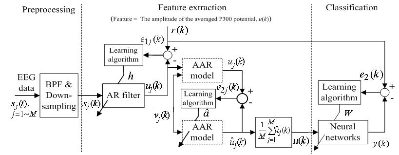Figure 3. Structure of the proposed feature extraction and classification algorithm

For the completion of the work, how the data were made in[3] is briefly summarized below. A six-choice signal paradigm was used to test a population of four disabled and four able-bodied subjects. Subjects 1 and 2 were able to perform simple, slow movements with their arms and hands but were unable to control other extremities. Spoken communication with subjects 1 and 2 was possible, though both subjects suffered from mild dysarthria. Subject 3 was able to perform restricted movements with his left hand but was unable to move his arms or other extremities. Spoken communication with subject 3 was impossible. However, the patient was able to answer yes/no questions with eye blinks. Subject 4 had very little control over arm and hand movements. Spoken communication was possible, though a mild dysarthria existed. Subject 5 was able to perform only extremely slow and relatively uncontrolled movements with his hands and arms. Communication was very difficult, due to severe hypophonia and large fluctuations in alertness. Subjects 6-9 were Ph.D. students (all males, aged 30±2.3 years), none of whom had any known neurological deficits.

In their test, four seconds after a warning tone, six different images (a television, a telephone, a lamp, a door, a window, and a radio) flashed in random order (one image at a time), and the subjects were asked to count silently the number of times of the flashes of a preselected image on the screen. The EEG signals were recorded, at 2048 Hz sampling rate, with the 32 electrodes placed at the standard positions described in the 10-20 International System[3],[35]. Each image flash was of 100 ms duration, followed by a 300 ms blank screen (i.e., the inter-stimulus interval was 400 ms). Each subject completed four recording sessions. The first two sessions were performed on a given day, the last two sessions on another day. The lapse between the first and the last sessions, for all of the subjects, was less than two weeks. Each of the sessions consisted of six runs, one run for each image. The duration of one run was approximately one minute and that of one session, including the time required for electrode setup and short breaks between runs, was about 30 min. One session averaged 810 trials, and the entire data for one subject, therefore, was taken from an average of 3240 trials.

Prior to feature extraction, several preprocessing operations including filtering and down-sampling were applied to the data. To filter the data, a 6th-order band-pass filter (BPF) with cutoff frequencies of 1 Hz (i.e., to remove the trend from low frequency bands) and 12 Hz (i.e., to remove unimportant information from high frequency bands) was used. Then, the signal was down-sampled from 2048 Hz to 32 Hz (i.e., satisfies the Shannon-Nyquist sampling theorem criterion) by selecting the first data of each 64th sample from the filtered data, which was considered sufficient to reduce unimportant information from high frequency bands. Extractions of single trials of 1000 ms length, starting at the stimulus onset (i.e., at the beginning of the intensification of an image), subsequently were performed. Due to the ISI of 400 ms, the last 600 ms of each trial were overlapping with the first 600 ms of the following trial.

3. Feature Extraction and Classification

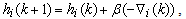
Each data set includes EEG data, events information, stimuli occurrence, target assignment, and target counting. The EEG data is of a matrix given by 34 rows the number of samples (columns), which reflects the data of 32 electrodes and 2 reference signals (average signal from the two mastoid electrodes was used for referencing). The dimension of a trial vector is M N, where M denotes 32 electrodes and N indicates the number of temporal samples of the trial. The goal of feature extraction is to find data representations that can be used to simplify the subsequent brain pattern classification or detection. The extracted signals should encode the commands made by the subject but should not contain noises or other interfering patterns (or at least should reduce their level) that can impede classification or increase the difficulty of analyzing EEG signals. For this reason, it is necessary to design a specific filter that can reduce such artifacts in EEG records. Thus, the AR-type is employed to adapt the coefficients of an FIR filter to match, as close as possible, the response of an unknown system[31-33].

In Figure 3, let denote the raw data of 2048 Hz, be the output of the BPF after down-sampling where k denotes the discrete time of 32 Hz, and represent the desired reference sequence in association with the given stimulus (target). Then, the filter output is given by

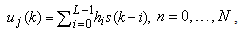(1)

where L and are the order and tunable coefficients of the filter, respectively. Let be the error between the reference signal and the filter output . The squared error is

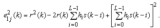(2)

The sum of the squared errors for N samples is given by[31-33]

(3)

where and are the cross-correlation function between the reference and preprocessed signals and the autocorrelation function of the preprocessed signal, respectively. They are defined as

(4)

(5)

To minimize (3), the steepest descent method[36] is employed. The adaptation law of the filter coefficient vector is expressed as follows.

(6)

where is a positive coefficient controlling the rate of adaptation, and the gradient is defined as

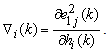(7)

Deriving (6) with respect to and replacing according to (1), we obtain

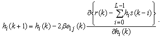(8)

Since and are independent of , (8) can be written as

(9)

where the term is the approximation of the negative of the gradient of the ith filter coefficients. This is the least mean squares recursive algorithm for adjusting the filter coefficients adaptively so as to minimize the sum of the squared error . Equation (1) with (9) represents the best model for , whose output is feasible as input to the adaptive autoregressive (AAR) model.

In the AAR model in Figure 3, a proper selection of its coefficients can represent the given signal well (in this paper, ). In minimizing the error, a proper updating algorithm and a proper model order are two important factors that need to be considered. The output of the AAR model is given in the following form[34]

(10)

where are the time-varying AAR model parameters, are the past p-samples of the time series where p is the order of the AAR model, and is a zero mean Gaussian noise process with variance . Here, it is assumed that the parameters change slowly in time. The past samples and the estimated AAR parameters are written as

(11)

(12)

The adaptive estimation algorithm for the parameters can be obtained as[34]

(13)

(14)

(15)

(16)

and

(17)

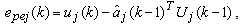
where is the one-step prediction error of the jth channels, and are the a priori and the a posteriori state error correlation matrix (p p), is the Kalman gain vector (1 p), is the identity matrix, and is the update-coefficient. If the estimates are near the true values (), the prediction error will be close to the innovation process , and the mean square error would be minimum. Through the estimated coefficients, the estimated output, , of the AAR model were obtained.

The artificial neural network has been employed in information and neural sciences for conducting research into the mechanisms and structures of the brain. This has led to the development of new computational models for solving complex problems involving pattern recognition, rapid information processing, learning and adaptation, classification, identification and modeling, speech, vision and control systems[25-30]. EEG signals in reality are generated by a nonlinear system comprising post-synaptic neurons firing action potentials; this makes the measured signals very noisy, and their classification performance is very poor. To overcome this problem, classification using an MNN is discussed in this subsection. Given a set of training samples , error back-propagation training begins by feeding all inputs through a multilayer perceptron network and computing the corresponding output , as shown in Figure 3 (here, the initial weight matrix W(0) is chosen arbitrary). The sum of the square error is then given by

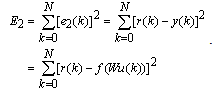(18)

The objective is to adjust the weight matrix to minimize the error . This becomes a nonlinear least squares optimization problem, and there are numerous nonlinear optimization algorithms available to solve it. These algorithms all adopt an iterative formulation similar to

(19)

where is the correction made to the current weight , which is solved using the steepest descend gradient method[37]. The derivative of the scalar quantity with respect to individual weights can be expressed as

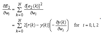(20)

where

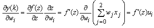(21)

Hence,

(22)

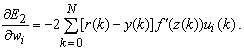
If is introduced, the above equation can be expressed

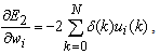(23)

where is the modulated error signal by the derivative of the activation function . The overall change is thus the sum of that correction over all the training samples. Therefore, the weight update formula takes the following form

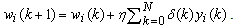(24)

If a sigmoid activation function is used, can be expressed as

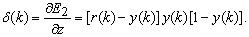(25)

Note that the derivative can be determined precisely without any approximation. Each of the weights updated time is called an epoch. In practice, the epoch size can be taken as the size of one trial. Here, the modified version of the weight update formula in (19) for training a multiple-layer neural network is presented. The net-function and output corresponding to the kth training sample of the jth neuron of the (Q-1)th layer are denoted by and , respectively. The input layer, being the zeroth layer, is given by . The output is fed into the ith neuron of the Qth layer via a synaptic weight denoted by or, for simplicity, . The weight adaptation equation is expressed as[37]

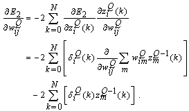(26)

In (26), the output can be evaluated by applying the kth training sample to the MNN with weights fixed to . However, the delta error term is not readily available, and so has to be computed. Note that is fed into all neurons in the (Q+1)th layer; hence

(27)

Equation (27) is the error back-propagation formula that computes the delta error from the output layer back toward the input layer, in a layer-by-layer manner. With the given delta error, the weights are updated according to the following modified formulation of (19):

(28)

The second term in (28) is the gradient of the mean square error with respect to . The third term (the momentum term) provides a mechanism for adaptive adjustment of the step size. Both of the parameters (i.e., learning rate and momentum constant ) are chosen from the interval of[0 1]. The last term is a small random noise term that has little effect when the second and third terms have large magnitudes. When the training process reaches a local minimum, the magnitude of the corresponding gradient vector or the momentum term is likely to diminish. In such a situation, the noise term can help the learning algorithm leap out of the local minimum and continue to search for the globally optimal solution.

It is difficult to compare performances of BCI systems, because the pertinent studies have derived and presented the results in different ways. Notwithstanding, in the present study, the comparison was made on the bases of accuracy and transfer rate. Accuracy is perhaps the most important measure of any BCI. Accuracy greatly affects the channel capacity and, thus, the performance of a BCI. And if a BCI is to be used in control applications (environmental controls, hand prosthetics, wheelchairs, etc.), its accuracy is, obviously, crucial. One needs only to imagine a wheelchair lacking controllability in the street. Besides accuracy, the transfer rate also is very important. The transfer rate (bits per minute) or speed of a particular BCI is affected by the trial length, that is, the time required for one selection. This time should be shortened in order to enhance a BCI’s communicative effectiveness. When considering using a BCI as a communication or control tool, then, it is important to know how long it takes to make one selection. Although a classification can be made in a short time interval, one selection cannot necessarily be made in that same time.

BCI performance can be evaluated from the standpoint of (i) speed and accuracy in specific applications or (ii) theoretical performance measured in the form of the information transfer rate. The information transfer rate, as defined in[38], is the amount of information communicated per unit of time. The transfer rate is a function of both the speed and the accuracy of selection. The bits (bits/trial) can be used in comparing different BCI approaches or for measuring system improvements[8]. The bits ([3],[15],[16]) of a BCI with mental activities in its controlling set and a mean accuracy P (i.e., 1 − P is the mean recognition error), is given by

(29)

The transfer rate is equal to the bits multiplied by the average speed of selection trial per minute (i.e., the reciprocal of the average time required for one selection).

4. Results and Discussions

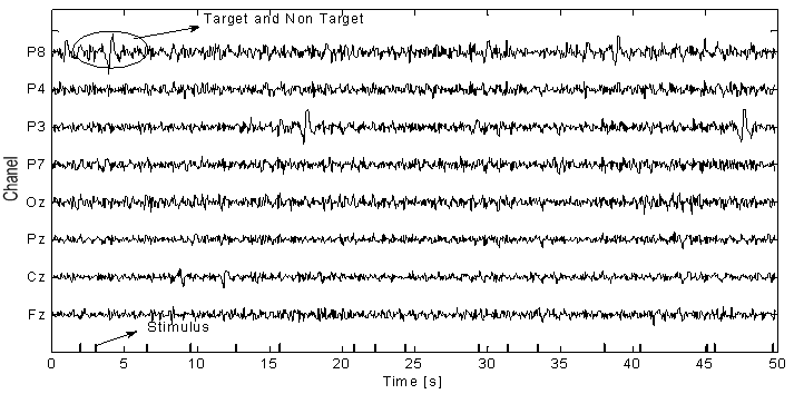
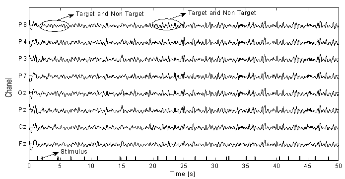
The EEG signals were first preprocessed using a sixth-order band-pass filter with cut-off frequencies of 1 Hz and 12 Hz, respectively, see Figure 4. It can be seen that the signals were corrupted by noises. The feature extraction of the pre-processed signals of the eight electrodes (Fz, Cz, Pz, Oz, P7, P3, P4, and P8) has been compared for three cases: i) using only the AR filter, ii) Using only the AAR model, and iii) the proposed combination of both. In obtaining Figures 5-7, the first half of the first three sessions out of 4 sessions of a trial was used for training (i.e., the half for validation).

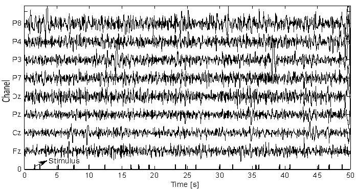Figure 4. EEG signals preprocessed using the BPF

Figure 5. Feature extraction using only the AR filter (w/o the AAR model)

Figure 6. Feature extraction using only the AAR model (w/o the AR filter)

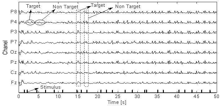Figure 7. Improved feature extraction using the combination of the AR filter and AAR model

Then, the optimal coefficients obtained in 3 sessions were used for testing the last session. The used adaptation step size β of the AR filter in (9) was 0.95, and the model order p in (12) and the update coefficient v in (15) of the AAR model were 6 and 0.0065, respectively. Figures 5 and 6 show the feature extraction results of the individual AR filter and AAR model, respectively. The features were extracted every 400 ms interval for about 126 target trials. Although there is some noticeable improvement, it remains difficult to identify the associated signals with respect to the given stimulus. In order to track the dominant waves, the combination of the AR filter and AAR model is demonstrated in Figure 7. In this scheme, the signals extracted by the AR filter were used to estimate the AAR parameters at each time. From the results in Figure 7, although the signals were still corrupted by noises (i.e., marked with high amplitude of non-target at some trials), the behaviours of the extracted signals clearly represent the EEG-based P300 evoked potentials (i.e., marked with higher amplitude of the target).

The ability to measure and classify single-trial responses from specific brain regions has important theoretical and practical implications for both basic and applied research. For brain research, the ability to measure single-trial EPs is an important step toward understanding how the relative timing of neuronal activity affects learning and how the memory of a particular experience can be encoded rapidly with a single or very few exposures. In clinical applications, the ability to obtain such measures in a computationally efficient manner could allow for functionally meaningful brain signals to be extracted and used to generate better input and feedback signals for BCIs. In the present study, a MNN based on a back-propagation training algorithm classifier is employed. In the three-layer neural network classifier, the input layer consists of a number of neurons equal to the six selected features. The hidden layer has a variable number of neurons. The output layer consists of one neuron, which encodes the target. The back-propagation algorithm with an adaptive learning rate and momentum was used to train the neural networks. The values of the learning rate and the momentum were estimated by trial and error until no further improvement in classification could be obtained. The parameter values chosen were 0.3 and 0.8, respectively. The initial weights of the neurons were arbitrary selected within the[–1, 1] range. The log-sigmoid and tan-sigmoid activation functions were used for the hidden and the output layers, respectively. The appropriate number of hidden neurons was estimated according to the formula[39], where q is the number of neurons of the input layer and s the number of neurons of the output layer. In order to avoid overtraining and to achieve an acceptable generalization in the classification, three data sets were employed: a training set, a validation set, and a testing set. The neural network was trained using the training set (three sessions in the first evaluation and two sessions in the second evaluation), whose phase was completed when the performance for the validation set was maximized. The generalizability was tested using the testing set containing samples that had not been used previously. The performance was measured according to the specified performance function (i.e., mean square error). The convergence of the mean square errors to zero (using y(n): with proposed method and x(n): without proposed method, see Figure 8) verified the performance of the network with the proposed feature extraction method. Specifically, the curves show that by application of feature extraction, an acceptable level of accuracy was attained after about 500 iterations. However, without feature extraction, the same level of accuracy, after 1800 iterations, was the able-bodied subjects, indicating that the recorded signals from the former were more corrupted.

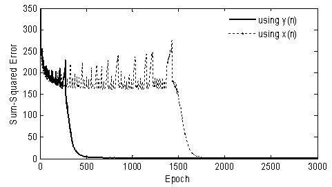Figure 8. Reduction of MNN training time by using the proposed feature extracted method

The data sets for subject 5 were not included in the simulation, since he had misunderstood the pre-experiment instructions[3]. Comparative plots of the classification accuracies and transfer rates (obtained with and without the proposed feature extraction method and averaged over three sessions training) for the disabled (subjects 1 – 4) and able-bodied subjects (subjects 6 – 9) are provided in Figures 9 and 10, respectively. All of the subjects achieved an average classification accuracy of 100% after four blocks of stimulus presentations were averaged (i.e., 10 sec). This represents a significant improvement compared with the results presented in[3], in which subject 6 and subject 9 failed to achieve 100% average classification accuracy. In Tables 1 to 4, the improvement for each subject is calculated by subtracting the fifth column (for Tables 1 and 3) and the third column (for Tables 2 and 4) with the second column, respectively. The improvement for the averages is calculated by averaging S1-S4, S6-S9, and S1-S9, and its variances, respectively. Shown alongside the classification accuracies for all of the subjects, in Table 1, are the corresponding 97% confidence intervals. According to Table 1, subject 1 showed the best improvement (9.2%) of average classification accuracy over all of the experiments. By contrast, subject 7 showed the worst improvement (1.45%). If we analyze the results for both accuracy and transfer rate (see Tables 1 to 4), the disabled subjects obtained better performance improvements both with and without the proposed feature extraction method. These results reflect the fact that the brain signals of the disabled subjects were less noisy and more homogeneous than those of the able-bodied subjects.

Table 1. Average classification accuracy over three sessions training (%) Subject Preprocessing AR Filter AAR Model AR filter + AAR Model Improvement S1 89.8 95.25 97.00 99.00 9.20 S2 90.8 95.5 96.50 99.05 8.25 S3 96.5 97.75 97.75 99.25 2.75 S4 95.9 96.0 97.75 98.75 2.85 S6 92.5 94.25 93.15 97.40 4.9 S7 96.5 97.3 96.00 97.95 1.45 S8 97.1 97.9 97.00 99.10 2.00 S9 94.1 96.6 95.55 98.85 4.75 Average (S1–S4) 93.8±4 96.1±1 97.2±0.6 99.0±0.2 5.7±3.4 Average (S6-S9) 95.0±3 95.5±2 95.4±1.6 98.3±0.7 3.2±1.8 Average (all) 94.9±3 96.3±1 96.3±1.5 98.6±0.6 4.5±2.8

Table 2. Average classification accuracy over two sessions training (%) Subject Preprocessing AR Filter + AAR Model Improvement S1 87.75 95.0 7.25 S2 91.5 94.0 2.50 S3 94.25 98.0 3.75 S4 89.0 96.5 7.50 S6 77.0 90.75 13.75 S7 89.25 95.5 6.25 S8 89.5 96.0 6.50 S9 92.0 94.0 2.00 Average (S1–S4) 90.63±2.88 95.88±1.75 5.25±2,51 Average (S6-S9) 86.94±6.74 94.06±2.37 7.12±4.87 Average (all) 88.78±5.19 94.97±2.16 6.19±3.73

Comparisons of the classification accuracies and transfer rates averaged over two sessions training for the disabled and able-bodied subjects are plotted in Figures 11 and 12, respectively. All of the subjects achieved an average classification accuracy of 100% after about six blocks of stimulus presentations were averaged (i.e., 14 sec). These results still represent significant improvement compared with those presented in[3], where the classification accuracies were obtained over three sessions of training. Shown alongside the classification accuracies for all of the subjects, in Table 2, are the corresponding 94% confidence intervals.

Table 3. Maximum average transfer rate over three sessions training (bits/min) Subject Preprocessing AR Filter AAR Model AR Filter + AAR Model Improvement S1 12.48 20.95 34.97 40.67 28.19 S2 13.04 25.18 29.83 40.67 27.63 S3 34.97 34.97 34.97 48.49 13.52 S4 25.18 17.13 29.83 47.09 21.91 S6 19.38 25.18 13.68 33.90 14.52 S7 32.31 34.97 34.97 34.97 2.66 S8 44.42 40.67 34.97 47.10 2.68 S9 26.98 29.83 25.18 47.10 20.12 Average (S1–S4) 21.4±10 24.5±7.6 32.4±2.9 44.2±4.1 22.8±6.8 Average (S6-S9) 32.2±11 32.6±6.6 27.2±10 40.7±7.3 9.9±8.7 Average (all) 26.8±11 28.6±7.9 29.8±7.4 42.5±5.8 16.4±9.9

The transfer rates corresponding to the MNN classification accuracies for the eight-electrode configuration were tested. The results showed that significant improvements in both classification accuracy and average transfer rate were obtained. The maximum average transfer rates, the mean transfer rates, and the standard deviations for all combinations of the feature extraction algorithm are listed in Table 3 (three sessions training) and Table 4 (two sessions training), respectively. These results show that the maximum average transfer rates for all of the subjects were much better with the proposed feature extraction method. These improvements can be seen in the last column of each table. In the work of Hoffmann et al. (2008), the maximum average transfer rate was about 15.90 bits/min for disabled subjects and 29.30 bits/min for able-bodied subjects, respectively. In the present study, improvements in the maximum average transfer rates were achieved for the same electrode configuration: 48.49 bits/min for the disabled subjects and 47.10 bits/min for the able-bodied subjects. This confirmed the BCI-applicability of the proposed combined method. By contrast, the classification accuracies and transfer rates obtained using the AR filter and AAR model approaches separately were found to be only marginally superior to mere chance, indicating the inadequacy of those methods for BCI applications.

Table 4. Maximum average transfer rate over two sessions training Subject Preprocessing AR Filter + AAR Model Improvement S1 9.23 25.18 15.95 S2 11.77 12.93 1.16 S3 15.70 34.97 19.27 S4 11.65 25.18 13.53 S6 5.30 10.60 5.30 S7 12.59 25.18 12.59 S8 10.60 34.97 24.37 S9 15.18 17.13 1.95 Average (S1–S4) 12.09±2.67 24.56±9.02 12.47±7.90 Average (S6-S9) 10.92±3.18 21.97±10.51 11.05±9.92 Average (all) 11.50±2.96 23.27±9.17 11.77±8.34

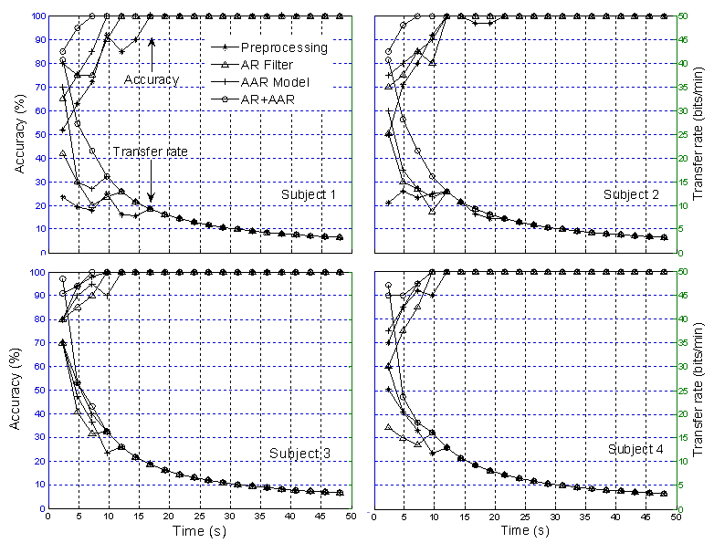Figure 9. Comparison of classification accuracy and transfer rate: Based on three sessions training for disabled subjects

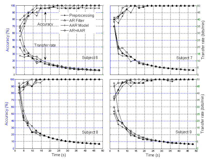Figure 10. Comparison of classification accuracy and transfer rate: Based on three sessions training for able-bodied subjects

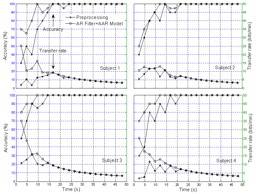Figure 11. Comparison of classification accuracy and transfer rate: Two sessions training in MNN for disabled subjects (* the preprocessed signal and O the AR+AAR feature extraction)

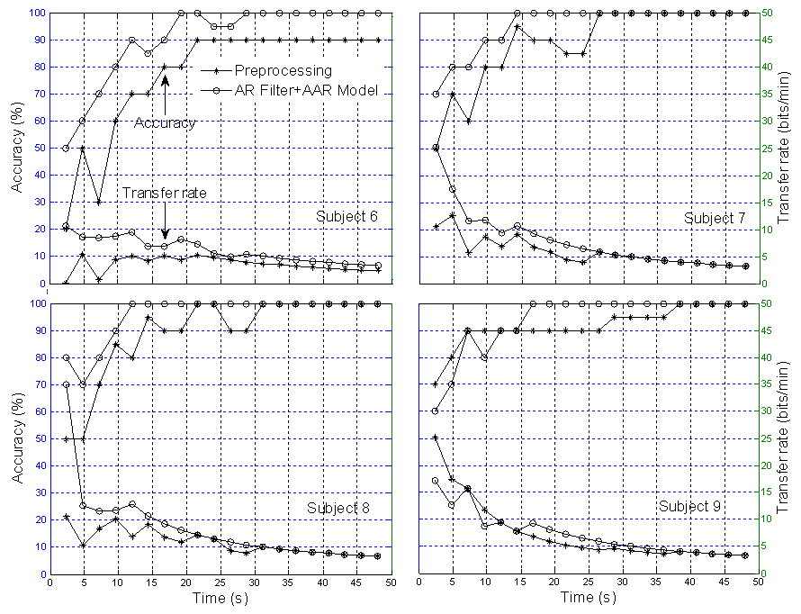Figure 12. Comparison of classification accuracy and transfer rate: Two sessions training in MNN for able-bodied subjects (* the preprocessed signal and O the AR+AAR feature extraction)

One negative characteristic of P300 detection is that the amplitude of the waveform requires the averaging of multiple recordings to isolate a signal. In the present study, in order to streamline the averaging process, the proposed method’s feature extraction modules were applied to segments of EEG signals (EEG trials). These modules are integral to the classification accuracy and transfer rate of the mental activities. A factor relating to the attainment of good classification accuracy and transfer rates for disabled subjects, both in communication systems and BCI systems, is the sequence of a given stimulus. When applying the proposed method to extract EEG signal features, it was found that any two sequential target stimuli excite just one P300 component peak, and are extracted in that form. However, in order that EEG signals be classified with 100% accuracy, such stimuli must excite two peaks of amplitude. Therefore, in order to obtain a good classification accuracy and transfer rate, the given stimulus must be inputted randomly with a constraint. In other words, two targets should not be flashed sequentially.

5. Conclusions

The feature extraction method introduced in this study showed how a better extraction result can be obtained when using the multilayer neural network (MNN) algorithm for single-trial EPs based on the P300 component from specific brain regions. An average 100% classification accuracy was achieved, both for four blocks over three sessions training and six blocks over two sessions training. With regard to the classification accuracy, the data indicates that a P300-based BCI system can communicate at a rate of 48.49 bits/min for disabled subjects and 47.10 bits/min for able-bodied subjects, respectively. The classification and transfer rate accuracies obtained using the AR filter and AAR model approaches separately were found to be only marginally superior to mere chance, indicating that neither approach is adequate for BCI applications. However, with the combined AR filter and AAR model method, the classification and transfer rate accuracies were far superior and, moreover, entirely BCI-implementable.

ACKNOWLEDGEMENTS

This research was supported by the tematic program (No. 3425.001.013) through the Bandung Technical Management Unit for Instrumentation Development (Deputy for Scientific Services) and the competitive program (No. 079.01.06.044) through the Research Center for Metalurgy (Deputy for Earth Sciences) funded by Indonesian Institute of Sciences, Indonesia.