1. Introduction

Deforestation and degradation of tropical forests constitute the second largest source of anthropogenic emissions of carbon dioxide after fossil fuel combustion (Van der Werf et al. 2009). Policy initiatives have been proposed to reduce the rate of tropical forest loss, which would have the benefit of preserving other unique tropical ecosystem services such as biodiversity richness (Jantz, et al 2014).

The flux of carbon in the atmosphere from tropical land-use change is one of the largest uncertainties in the contemporary carbon budget (Schimel et al. 2001), because of the difficulties in quantifying deforestation and regrowth rates, initial biomass, and fate of carbon in areas where vegetation has been cleared. Suggested schemes for carbon credit incentive based on deforestation (Mollicone et al. 2007) or carbon stock baselines (Gurney and Raymond 2008) require accurate estimates of biomass (Baccini et al. 2008). Also an accurate biomass estimation is required for the implementation of a reliable REDD+ mechanism under the United Nations Framework Convention on Climate Change (UNFCCC) (Gibbs et al. 2007a). While, there is high interest in seeing such initiatives take form, monitoring forest biomass stocks and stock changes is identified as a key challenge for developing countries wishing to take part in the expected REDD+ mechanism (Herold and Skutsch 2011).

In order to respond to the problem of deforestation and forest degradation, Togo joined the REDD+ mechanism, in particular the Forest Carbon Partnership Facility (FCPF) through resolution PC/16/2013/9 in 2013 and then to the UN-REDD program in 2014, because of the decision 3.1 of its orientation council. Since 2015, Togo has been implementing its readiness proposal measures for REDD+ (R-PP).

Despite its degraded state, the semi-deciduous forest zone of Togo which extends over the plateau and central region of Togo is one of the main carbon sink in the country (MERF 2016). However, monitoring the biomass changes by remote sensing in the semi-deciduous forest zone of Togo is a challenge because, of the effect of the landscape and different forest types that mix up with fallows and secondary forests growing on agricultural land. Moreover, biomass estimation at the landscape level are necessary for understanding processes of the target landscapes and provide baseline data for future studies (Foody et al 2003; Woodcock et al. 2001; Zheng et al. 2004). The ability to map forest biomass is thus important for monitoring changes in forest structure and changes in the carbon account (Labrecque et al. 2006). These facts therefore raise a research question: What aboveground biomass can be observed spatially in the study area over the last decades?

In the context of REDD+ in Togo, previous work on forest cover mapping has provided valuable insight into vegetation status and different maps were produced (MERF 2018). However, few data are available on forest biomass mapping and no data are available on forest biomass change mapping. Indeed, in 2016, the World Bank funded the definition of the methodology and tools for biomass estimating in various compartments in Togo (MERF 2017). Despite the production of biomass map for the year 2015 (Dangbo et al. 2020) based on the first national forest inventory realized in 2015/2016, further improvements in classification methods for biomass change are necessary in order to provide accurate and consistent estimates of biomass change at national and subnational levels. According to Houghton (2005), it is critical to have reliable and current information on the spatial distribution of AGB in the forest’s zone over the last decades for calculating the sources (and sinks) of carbon that result from converting a forest to cleared land (and vice versa) and to enable measurement of change through time.

In recent decades, efforts have been made to estimate forest biomass, including field measurements and model simulations. Numerous regression models have been developed to estimate AGB (Chave et al. 2009; 2014) while these models are accurate at tree, plot, and stand levels, they are limited when considering spatial pattern analysis of AGB across the landscape (Zheng et al. 2004). Models derived from remote sensing need further calibration with ground data before they can be used appropriately to predict AGB for a given landscape. It has been demonstrated that the Landsat imagery is very useful for monitoring environmental change when combined with field measurements (Dorren et al 2003; Woodcock et al. 2001). This highlights a research question: How can aboveground biomass changes be mapped consistently, in areas with high forest dynamics?

The general objective of the study is to contribute to the monitoring of biomass dynamics in the context of REDD+. The specific objectives of this work is to combine national forest inventory and remote sensing data to: (1) develop a model to estimate aboveground biomass (AGB) over the last 30 years and (2) analyze changes in aboveground biomass during that period.

2. Materiel and Method

2.1. Study Area

The study area corresponds to Togo’s bioclimatic region “ecological zone IV” and is located in the southern part of the Atakora mountains, south-west of Togo, on the border between Togo and Ghana in the region called Togo Mountains or Togo highlands. The studied area extends between the latitude 6° 15 and 8° 20 and the longitude 0° 30 and 1° and covers an area of 603’972 hectares (Figure 1). The climate prevailing in this area is a Guinean mountain climate characterized by a long rainy season (8-10 months). The average annual temperature varies from 21° to 25°C and the total annual rainfall ranges varies from 1400 to 1700 mm. This zone contributes significantly to species richness in Togo (Adjossou 2009). It is the current domain of semi-deciduous forests. The study area shows a strong topographic heterogeneity. The average altitude is 800 m, with peaks at Djogadjèto (972 m) and Liva (950 m). A succession of plateaus (plateau of Kloto, Kouma, Danyi, Akposso, Akebou and Adele) where hills along with their valleys and caves are common. Landforms are diverse and complex. The main geologic component is of the late Precambrian: Togo and Buem quartzites phyllites, shales and sandstones were largely folded and metamorphosed during the Cambrian Pan-African Orogeny (Hall and Swaine 1976). A network of complex secondary rivers covers the area with three catchment areas: the basin of the lake Volta in the west of the Mounts and basins of the Mono River and Zio River in the east of the mounts. Population distribution and land management varies across the area with implications for forest cover changes.

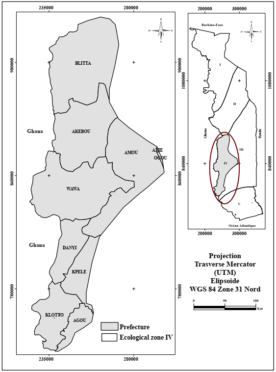Figure 1. Study area

2.2. Overview of Data and Methods

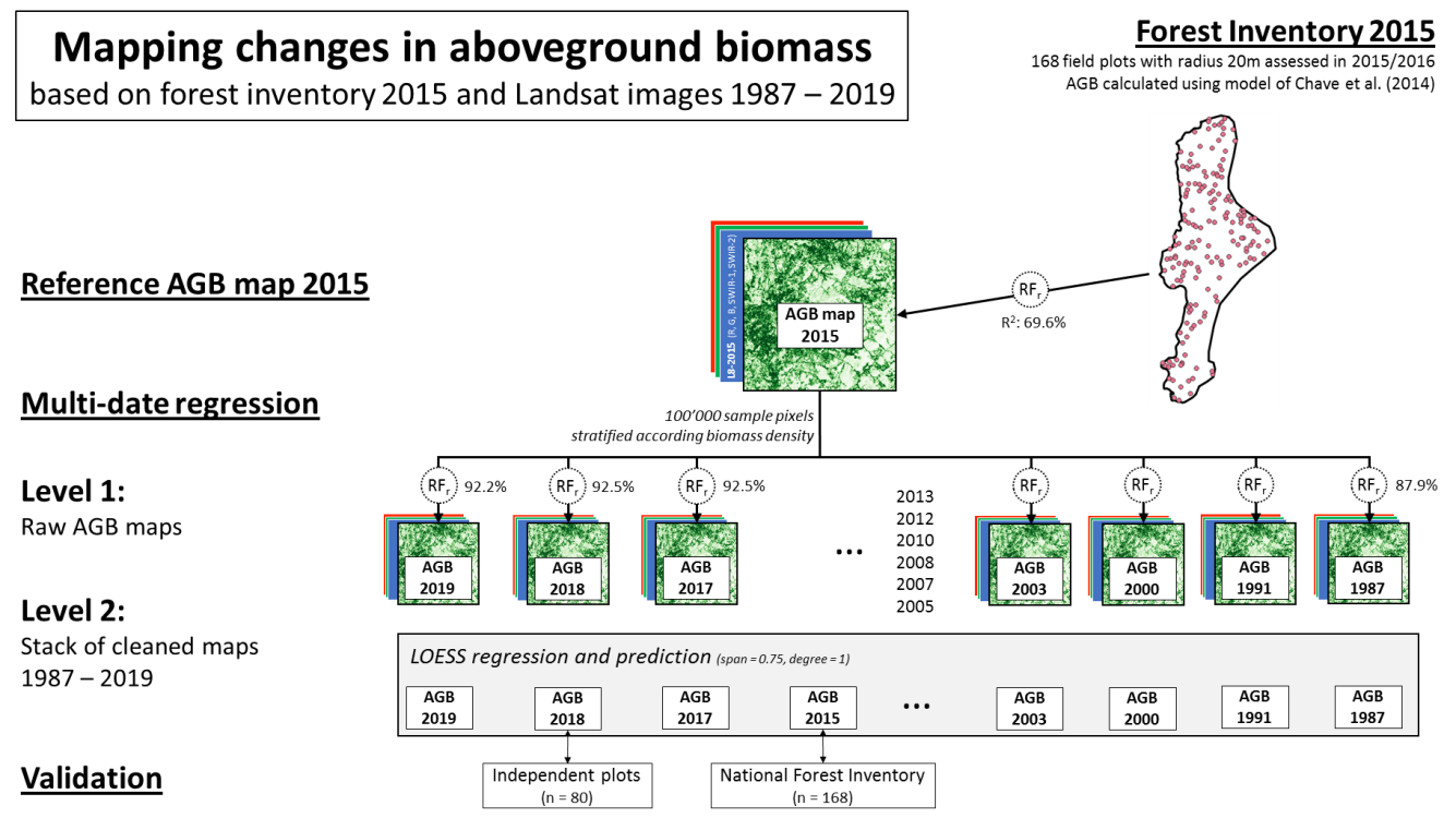
The steps of this research are: (a) acquisition, preprocessing, and stacking of Landsat images, (b) AGB estimated based on national forest inventory data (Dangbo et al 2019) (c) classification of reference biomass map 2015 based on AGB calculated and using RandomForest (Dangbo et al 2019), (d) Biomass classification of Landsat time series based on reference maps, again using RandomForest, (e) cleaning of time-series using majority filters and (f) accuracy assessment of resulting maps using a set of independent and national forest inventory validation plots. These steps are outlined in Figure 2.

2.2.1. Landsat Image Collection and Pre-Processing

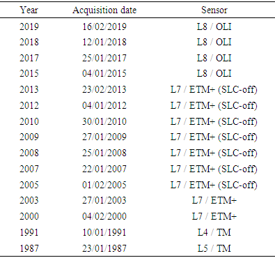
Landsat's temporal and spatial coverage, moderate spatial resolution, and long history of earth observations provide a unique opportunity for characterizing vegetation changes across large areas and longtime scales (Pflugmacher et al. 2014). A number of other national biomass maps have been produced based on the analysis of full coverage of Landsat data (Pflugmacher et al. 2014; Ji et al. 2012; Labrecque et al. 2006).

The study area is covered by two WRS2 scenes with path 193 and rows 054 and 055. Landsat surface reflectance data at the end of the dry period (Jan - Feb) with less than 10% cloud cover were downloaded from the U.S. Geological Survey (USGS) Center for Earth Resources Observation and Science (EROS) portal (https://earthexplorer.usgs.gov/) at full spatial and spectral resolution (30 x 30 m resolution).

The final dataset obtained consists of a series of 15 geometrically and radiometrically corrected images from satellites Landsat 4 and 5, Landsat 7 and Landsat 8, covering a period of 32 years (Table 1). According to Gutman et al (2008), these data have satisfactory radiometric and geometric qualities for performing land-use change analyses and in particular the historical analysis of deforestation. Due to problem with the sensor (Scan Line Corrector or SLC) since 2003, the Landsat 7 images of the years 2005 to 2013 have high rates of missing data (leaf stripping) even if it’s have good geometric and radiometric qualities (Barsi et al. 2007).

Table 1. Acquisition date and sensor of Landsat images used for historical analysis of biomass change between 1987 and 2019. The covered WRS2 scenes are p193r054 and p193r055

For each date, the six spectral bands B, G, R, NIR, SWIR1 and SWIR2 of the Landsat images of scenes p193r054 and p193r055 were mosaicked and projected to the coordinate reference system WGS 84 - UTM 31. All data processing and analysis of satellite images were done using the R environment for statistical computing (R Core Team 2013) using the R-packages “raster” (Hijmans 2019).

2.2.2. Production of Aboveground Biomass Map

A conceptual framework was developed to show the main steps in the production of the aboveground biomass reference map and the map of changes in aboveground biomass using field data and satellite information (Figure 2). The 2015 above-ground biomass calculated on the basis of the national forest inventory as well as images from 2015 were integrated into the "Random forest" algorithm to produce the 2015 biomass aerial map (Dangbo et al. 2020). This 2015 biomass map was used as a reference for producing the biomass map for all 15 dates between 1987 - 2019. This was done by selecting 100,000 pixels of samples, distributed over 50 carbon density classes. Then, the RandomForest algorithm was used to find the regression between the AGB of these 100000 pixels in 2015 with the spectral values in the other dates of the series. The resulting model was applied to produce the AGB maps for the different dates. In order to extract trends and make the noises go out, series of AGB maps produced were smoothed over time with a sliding spline (LOESS with parameters span = 0.75 and degree = 1) before starting the analysis of changes in the aboveground biomass.

Figure 2. Diagram of AGB and AGB Change Modeling from 1987 to 2019

2.2.3. Model Validation

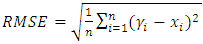
Validation of Landsat-based biomass estimates for the year 2015

The Landsat-based biomass of the year 2015 generated from the model was validate based on the national forest inventory for the year 2015 (Dangbo et al. 2019). The accuracy of the model was assessed through both comparisons between the predicted AGB values and the measured AGB from the field. Three measurements were made to quantify accuracy: root mean square error (RMSE), relative RMSE (RMSEr) as a percent of the mean of the field inventory biomass, bias. RMSE is frequently used to assess the differences between values predicted by a model and the values observed or measured. It is defined as: where and are the predicted AGB and measured AGB of the ith plot respectively, and n is the total number of plots. The reliability of the biomass estimates was assessed according to the RMSE between the predicted and observed biomass and the associated bias. A smaller RMSE indicates a higher accuracy.

The relative RMSE (RMSEr) is define as RMSEr = (RMSE/y)*100 where y is the mean of the observed values. The bias of the model is calculated as: Bias = e1- e2 where e1 is the mean value of the estimated biomass and e2 is the mean value of the validation plots (Fazakas et al. 1999). The positive value of bias suggests an overestimate of AGB by the model, while negative value of bias indicate an underestimate of AGB by the model. The coefficient of determination (R2) shows how well observed AGB are predicted by the model, as the proportion of total variation of AGB explained by the model. In addition, the mean biomass and the corresponding standard deviations were calculated for each forest strata, allowing the determination of which strata are most sensitive to errors (Dangbo et al. 2019).

Validation of biomass change

Changes in above ground biomass between different dates cannot be quantitatively validated due to a lack of inventory data in the past. The plausibility of changes in above-ground biomass observed on the maps was tested by comparing the observed dynamics with the expectations of people familiar with the reality on the ground. Moreover, we compared the forest cover map from Dangbo et al. (2020) studies with the produced biomass map to assess if there is a correlation between the biomass and the forest stand. These comparisons provide strong support for the validity of the approach and associated map.

In order to further evaluate the accuracy of the produced maps, the 2018 biomass map was cross-mapped to the forest cover change map (1991-2018) produced by Dangbo et al. (2020). The purpose of this cross is to correlate classes of forest cover change between the period 1991-2018 and biomass in 2018 and characterize classes of change in terms of above-ground biomass.

2.2.4. AGB Variation over Forest Change Area

To evaluate AGB change over forest area, we crossed the forest cover change map from 1991 to 2018 and the biomass change map from 1991 to 2018 to estimate the AGB loss due to deforestation (Forest loss/ AGB loss) and AGB loss due to degradation (Stable forest/ AGB loss). The total area of AGB considered only consider the variation of AGB in the area which was forest in 1991. To estimate AGB loss due to forest degradation, we estimated changes in area of stable forest based on Dangbo et al (2020) forest cover change map and the approach developed by Tyukavina et al. (2013); Potapov et al. (2008) and Zhuravleva et al. (2013). All data processing, statistical analyses and Figures were created using R Statistical Software (R Core Team 2019).

3. Results

3.1. Validation of Modeled AGB of the Year 2015

Total biomass and mean biomass values calculated for the model in addition to the error estimations (Table 2) provided an indication of the errors inherent in the biomass map. The mean biomass estimated derived from the model ranged from 40.34 (savanna) to 118.71 (dense forest) Mg/ha. These values suggested that the biomass map underestimated biomass when compared with the field data plots, which had overall bias values of -2.8 (Mg/ha). All forest strata had negative bias, except for forest plantation and savanna. The lowest bias registered occurred for fallow strata (-2.77 Mg/ha). The model overestimated biomass for the two strata (Forest plantation and Savanna) and underestimated biomass for the remain forest strata (Fallow, Woodland, Dense forest and Gallery forest). The RMSE values ranged from 27.41 to 35.66 Mg/ha depending on the forest strata and the overall RMSE value is around 15 Mg/ha. The contribution of dense forest and gallery forest to the total above ground biomass was greater than those from all the other forest strata.

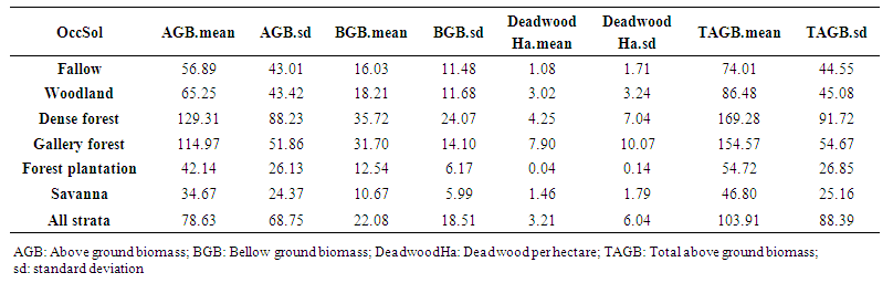Table 2. Biomass of each strata from the field: Source: First National Forest Inventory (MERF 2015; Dangbo et al 2019)

3.2. Correlation between Above Ground Biomass Map and Forest Cover Map

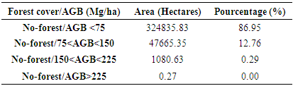
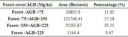
Crossing the forest cover 2018 and AGB 2018 maps showed a strong positive relationship between the forest cover map and the biomass map aggregated into 75 Mg / ha classes (Figure 3). The spatial AGB pattern on the AGB map primarily followed the distribution of the forest cover map. Indeed, 87% of no-forest area has AGB<75 Mg/ha and only 11% has forest with AGB < 75 Mg/ha (Table 3 and 4). These comparisons strongly validate the approach and associated maps.

Table 3. Discrimination of no forest area according to AGB (forest cover 2018 with biomass 2018 maps)

Table 4. Discrimination of forest area according to AGB (forest cover 2018 with biomass 2018 maps)

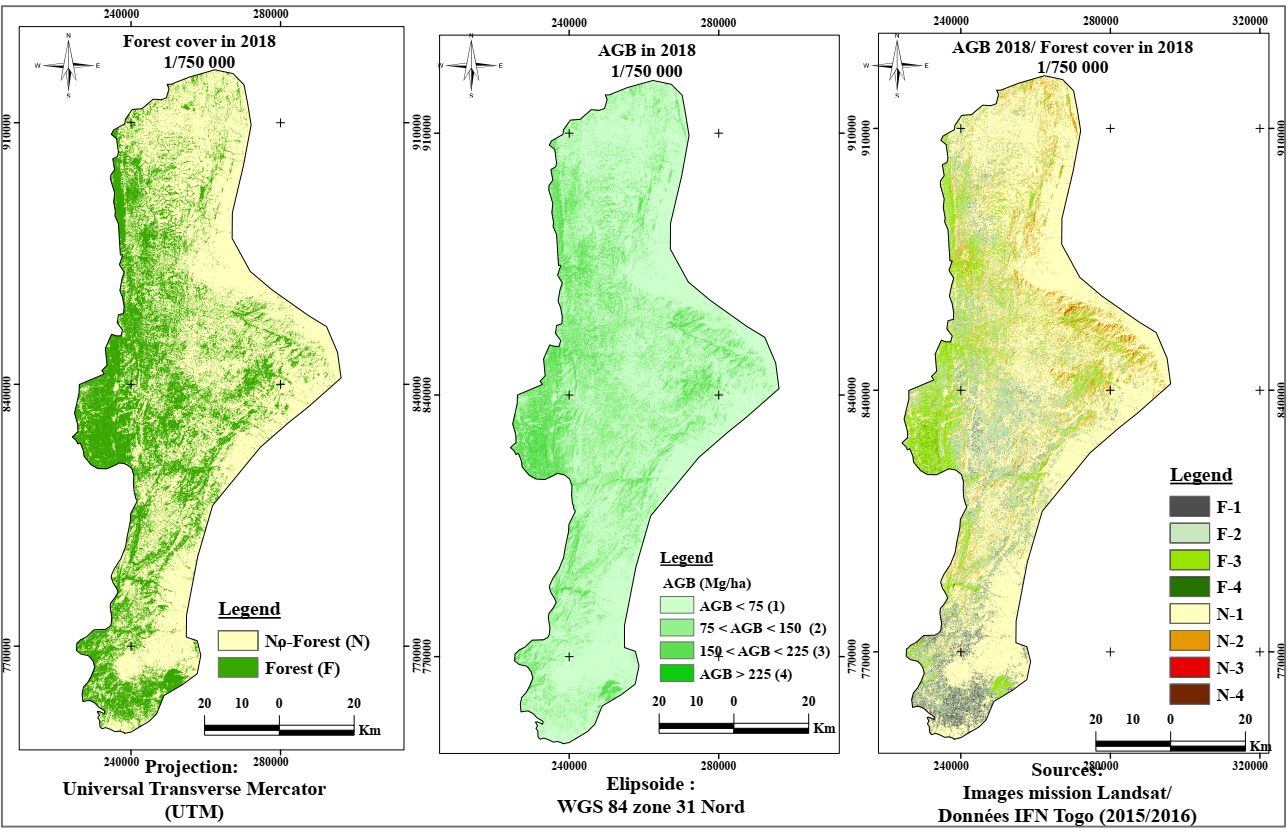Figure 3. From the left to the right: forest cover map, biomass map and crossing of forest cover and biomass

3.3. Distribution of Aboveground Biomass in Forest Area

When the AGB map was overlaid the forest cover map from Dangbo et al. (2020), result showed that in 2018, nearly 69% of forest’s area are distributed in savanna woodlands, woodland and dry forests that contain low biomass (AGB < 150 Mg ha−1) compared to 67% in 1991 (Figure 4 and 5). Low biomass density forests also include secondary forest, degraded forests and agroforest that are widespread forest zone. In 2018, 31% of forest have high biomass (150 225 Mg ha−1 in 2018 compared to 0.2% in 1991 (Figure 4 and 5).

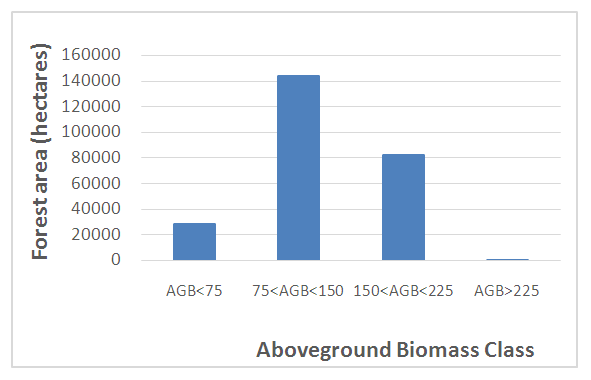Figure 4. Distributions of forest area (at 30% tree cover) for AGB class ranges of 75 Mg/ha in 1991

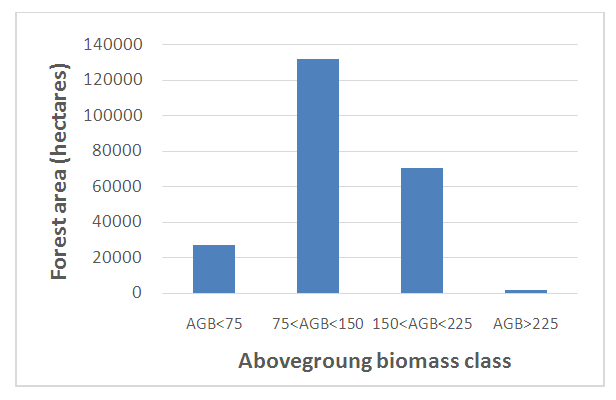Figure 5. Distributions of forest area (at 30% tree cover) for AGB class ranges of 75 Mg/ha in 2018

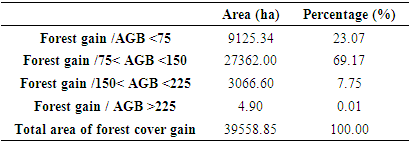
3.4. Status of Aboveground Biomass in Forest Cover Change Class

When the AGB map 2018 was overlaid the forest cover change map from Dangbo et al. (2020) result showed that 23% of the forest cover gain has low AGB (< 75 Mg / ha) and 69% has a AGB between 75 and 150 Mg / ha (Table 5).

Table 5. Discrimination forest gain area as a function of AGB (forest cover change for the period 1991-2018 with AGB 2018 map)

According to the result of this study (Table 6) forest loss is widely reported to have occurred in lands with low biomass: 48% forest loss occurred in land with Biomass <75 Mg/ha, being particularly prevalent in already fragmented agricultural landscapes. Moreover, 23.4% of forest loss occurred in land with biomass >225 Mg/ha (mature forests). We can conclude that the loss of forest with biomass < 75 Mg/ha was compensated by the gain of forest with the same biomass. However, the loss of forest with biomass > 225 Mg/ha was not compensated by the gain of forest with the same biomass.

Table 6. Forest loss area distribution for AGB class ranges of 75 Mg/ha in 1991 (before deforestation)

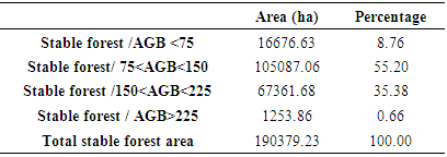
3.5. AGB Quantity in the Remaining Forest

The result of this study (Table 7), shows that almost 9% of stable forest (forest remain forest since 2019) have AGB <75 Mg/ha. More than 90% of stable forest have 75225 Mg/ha (Table 7). This result is showing that stable forest in view of forest cover change are land with few biomasses mainly degraded forest, new secondary forest.

Table 7. Stable forest area distribution for AGB class ranges of 75 Mg/ha

3.6. Evolution of Aboveground Biomass from 1991 to 2008

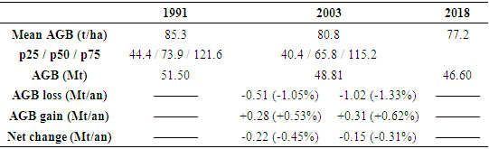
The result showed that between 1991 and 2003, there was an increase in formations with low biomass density (0 to 75 Mg / ha) (Figure 6). Forest formations with a low biomass density per hectare are fallows, forest recruits and young regenerations. During the same period, a regression of the formations having a density between 75 and 180 Mg / ha was observed. These formations correspond to moderately dense formations (degraded dense forest, clear forest, wooded savannas). Formations with a density between 180 and 225 increased slightly during this period. These formations correspond to dense forests, agro-forests or secondary forest / riparian forests. From 2003 to 2018, there was a regression of areas with very little biomass <25 Mg / ha, but a significant increase in formations with a density between 25 and 120 Mg / ha. This "increase" is associated with a decline in dense stands of 120 to 225 Mg / ha. During these two periods, formations with a biomass density greater than or equal to 250 Mg / ha are stable. These formations correspond to dense forests located in hard-to-reach areas and along streams.

The net annual rate of loss of aboveground biomass is estimated at 0.45% between 1991 to 2003 and 0.31% between 2003 and 2018 (Table 8). Biomass loss occurs in all types of forest formations over the area (Figures 6).

Table 8. Evolution of AGB and AGB change in the period 1991 and 2018

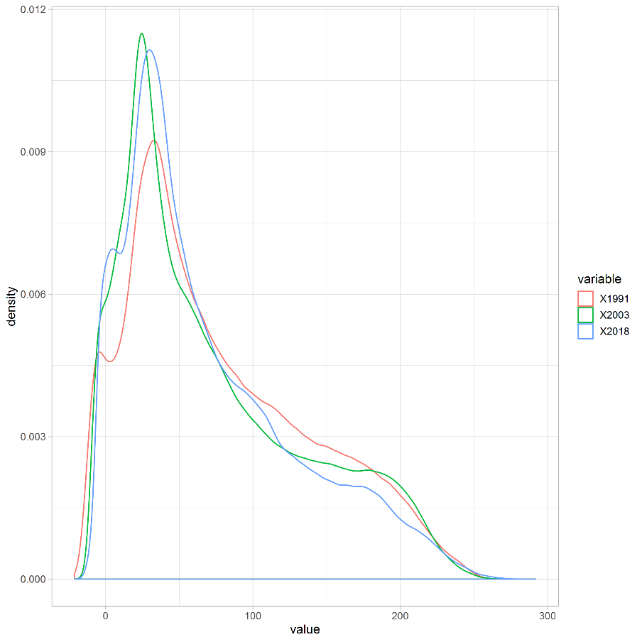Figure 6. AGB evolution in the forest’s zone in 1991, 2003 and 2018

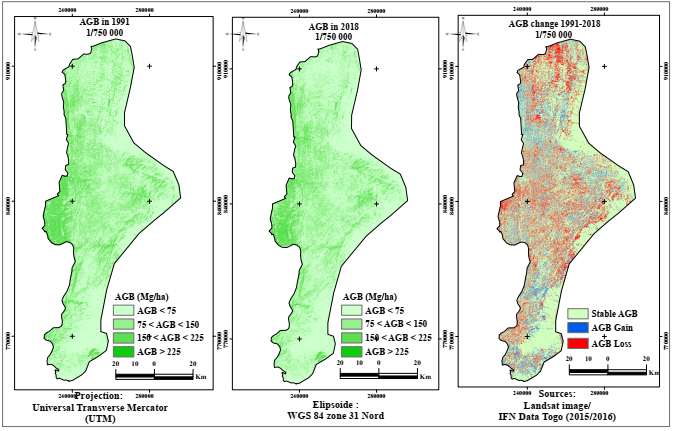Figure 7. From the left to the right: AGB map in 1991; AGB map in 2018; AGB map between 1991 et 2018

Table 8 shows that the mean AGB value for the studied area was 85.3 Mg/ha in 1991, 80.8 in 2003 and 77.2 in 2018. Based on the 25% and 75% quantiles (44.4 Mg/ha and 121.6 Mg/ha, respectively), 50% of the studied area had the AGB values between 44.4 Mg/ha and 121.6 Mg/ha in 1991. The AGB value decreased and in 2003, 50% of the studied area had the AGB values between 40.4 Mg/ha and 115 Mg/ha. The AGB map showed also, that the mean biomass decreases from 85,3 Mg/ha in 1991 to 77 Mg/ha in 2018 (Table 8).

3.7. AGB Change over Forest Change Area

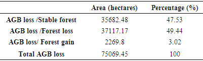
The result of crossing forest cover change map from 1991-2018 and the biomass changes map 1991-2018 showed that the total area of AGB loss between 1991 and 2018 is 75069 ha. Out of this, 47% of AGB loss is due to degradation (where forest is remaining forest: stable forest) and 49% of AGB loss due to deforestation (wholesale stand removals: forest loss).

Table 9. AGB loss distribution for forest cover change class for the period 1991-2018

4. Discussion

4.1. Model Validation

The results of this study demonstrate the utility of satellite data sets, for estimating above-ground carbon stocks even in areas with high forest dynamics. Moreover, Random Forest models are powerful for mining relationships in intensively sampled data sets (Baccini et al. 2008). Therefore, the most extensive field biomass data sets were used in a consistent fashion.

The results indicate that carbon losses exceed gains on the two periods. The average net AGB lost is 0.45% during the first period 1991-2003 and decreases to 0.33% during the second period 2003–2018.

The accuracies of the regression model and AGB estimates in 2015 are similar to previous studies that used optical remote sensing to map biomass. RMSE of models using multiple predictor variables in our study ranges between 27.41 to 35.66 Mg/ha and R² is 0.74. Labrecque et al. (2006) utilized Landsat TM images to map forest biomass in western New-foundland by four methods and reported results with RMSE around between 47 and 59 Mg/ha.

A comparison with forest cover map from Dangbo et al. (2020), where losses are concerned, we demonstrate clearly our sensitivity to reduction in AGB. The AGB loss in the first period 1991-2003 is very close to the forest lost in the same period (0.5%) according to Dangbo et al (2020). Unsurprisingly, the average per-hectare gains across the area tend to be lower because annual losses from deforestation and forest degradation are larger than gains from growth. Crossing forest cover map with the biomass map showed that biomass loss occurred widely in land with biomass < 75 Mg/ha. The mean AGB values by land cover type shows that the forests, had higher mean AGB values, while the no-forest had generally lower AGB. Zheng et al. (2004) found the same result when he showed that spatial patterns of AGB were clearly related to landscape structure and composition. For example, places with higher AGB are usually associated with mature forests, especially the hardwoods. Low estimates of AGB were often associated with young forests. The decreasing AGB trend was due to forest dynamic in the area.

4.2. Status of Forest Based on AGB Quantity

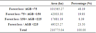
The result of this study showed that the semi-deciduous forest zone of Togo is very dynamic. The AGB change maps give more detail on change and disturbance at small scale mainly AGB loss due to degradation. In complement to forest cover change, AGB change map showed that the forest loss is more happened in small scale. Forest degradation processes that do not lead to the complete loss of tree canopy or cause small-scale canopy openings, result in significant AGB loss. Tyukavina et al. (2013) found the same result when he estimated the gross forest aboveground carbon loss in Democratic Republic of the Congo.

Furthermore, the result of this study showed that the quality of the forests lost and those gained are not always the same. Indeed, 92% of forest gain has AGB < 150 Mg/ha. This mean that forest gain is area with low to intermediate AGB mainly fallow, secondary forest. Only 0.01% of forest gain are mature forests (AGB > 225 Mg/ha). However, 23.4% of forest loss occurred in mature/dense forests. 48% forest loss occurred in land with Biomass <75 Mg/ha, being particularly prevalent in already fragmented agricultural landscapes. Forest lost are more fallows and secondary forest cleared in the agricultural cycle and continuously compensated with fallows on abandoned land elsewhere.

4.3. Implications for Togo REDD+ Strategy and Forest Monitoring

The precision and accuracy of our predictions meets the eligibility criteria of the IPCC for a MRV method i.e., with 20% of RSE (Houghton et al 2009).

The level of accuracy for which AGB mapping can and need to be observed with remote sensing to improve uncertainties of the global carbon balance is currently vague (Houghton et al 2009) and likely depends on how datasets are going to be used in carbon cycle models (Pflugmacher et al. 2014). The time-series approach apply in this study allows for annual trajectories of gains/losses in carbon storage to be generated at scales ranging from pixel to the study area. The main strengths of the method from a practical perspective is its compatibility with forest inventories and forest cover change mapping.

The utility of the presented approach under REDD+ comes from the fact that Landsat data are available globally free of charge. Landsat data may remain the most viable option for national-scale REDD+ monitoring for a number of countries (Tyukavina et al. 2015). Using Landsat data, we followed recommended good practice guidance on the use of map-based activity data.

According to Tyukavina et al. (2015), it is worth noting that the reference imagery for the sample based images may consist of high spatial resolution commercial data in place of Landsat, if resources for data acquisition and purchasing are available. In the case of Togo RapidEye image to map the reference map may improve the model. Landsat resolution assessments of forest change may lead to significant underestimation of forest carbon loss (Tyukavina et al 2013). The result of this study is a basis to estimate emissions from deforestation and forest degradation in the country. Indeed, to estimate emissions, we need to know the area of cleared forest and the amount of carbon that was stored in those forests (Gibbs et al. 2007b).

5. Conclusions

The biomass change was mapped at 30-m resolution for the forest’s zone in Togo using Landsat data and field measurements including tree, in both live and dead forms. In the study, we used a regression method to estimate regional AGB based on Randomforest and vegetation index that are closely related to biomass. Comparison of biomass and forest cover change maps showed strong positive correlations with the mapped biomass, and low standard errors across the full range of predicted AGB. The AGB map showed that the mean biomass decreases from 85,3 Mg/ha in 1991 to 77 Mg/ha in 2018. The spatial AGB patterns in this area are controlled primarily by forest cover dynamic. This is the first Togo’s forest zone biomass map based on satellite observations and forest inventory data. It provides not only important information on carbon stocks but an essential baseline for monitoring and modeling biomass over time in Togo at relatively high spatial resolution, toward the current political discussions on REDD+. Our results offer a great potential for increasing the understanding of forest structure and biomass distribution at a local scale. This information is necessary for obtaining more reliable carbon estimates and for better planning, management and conservation of these ecosystems. The AGB estimates for forest zone produced in this study will be a prototype for the national AGB mapping for Togo.

Results from this study have significant implications for policy initiatives like REDD+. The spatial scale of forest change characterization, reference information on forest type and carbon stock, and sample representativeness, can impact AGB loss estimation.

ACKNOWLEDGEMENTS

Thanks to the European Union (EU) program (AMCC/ PALCC) for partly funding this research, to those who helped to do the field work at the local grass route level and to those seeing the potential of the databases. We thank Nadia Solime TAOU for suggestions for improvement.