E. C. Merem 1, J. Wesley 1, S. Fageir 1, E. Nwagboso 2, M. Cristler 1, P. Isokpehi 1, C. Romorno 1, T. Thomas 1, S. Nichols 1
1Department of Urban and Regional Planning, Jackson State University, Jackson MS, USA
2Department of Political Science, Jackson State University, Jackson MS, USA
Correspondence to: E. C. Merem , Department of Urban and Regional Planning, Jackson State University, Jackson MS, USA.
| Email: |  |
Copyright © 2015 Scientific & Academic Publishing. All Rights Reserved.
Abstract
This paper examines the impacts of changing farm landscape in South Carolina low country using a mix-scale method of GIS and descriptive statistics with emphasis on the issues, environmental analysis of the trends and factors of change. While the results show gradual declines in farm land use elements with slight gains in some years, stressors such as fertilizer and agrochemicals remained widespread in a region with major risks to sensitive head waters and streams. With change attributed to a set of socio-economic variables, GIS mapping points to a gradual dispersal of ecological stressors and growing threats to the agricultural landscape and its ecosystem. To remedy the problem, the paper suggests the need for effective land use planning and zoning, periodic monitoring and assessment of hazards on the landscape followed by a regular use of GIS, the design of a regional information system and a new data infrastructure to optimize access to information. In absence of GIS and such a temporal-spatial framework to visualize the impacts, decision makers run the risk of prescribing policy change via faulty blueprints. The benefit of the research stems from the ability to pinpoint the risk of land resource deficits vital for future planning.
Keywords:
Assessment of change, GIS, South Carolina low country, Agricultural landscape, Factors of change
Cite this paper: E. C. Merem , J. Wesley , S. Fageir , E. Nwagboso , M. Cristler , P. Isokpehi , C. Romorno , T. Thomas , S. Nichols , GIS Assessment of Farm Landscape Change in South Carolina Lower Region, International Journal of Agriculture and Forestry, Vol. 5 No. 2, 2015, pp. 92-112. doi: 10.5923/j.ijaf.20150502.03.
1. Introduction
Over the last several decades in the United States, the South Eastern region continues to experience changing agricultural landscape at an alarming proportion. This is having serious impacts on the stability of the surrounding ecology of these states [1-4]. However, very little has been done to analyze the trends using a mix scale model of descriptive statistics and Geographic Information Systems (GIS) to visualize change across time and space. In absence of such a temporal-spatial framework, decision makers run the risk of prescribing policy change using faulty blueprints [5]. This paper will fill that void by focusing on the impacts of changing agricultural landscape in South Carolina low country using a mix-scale method of GIS and descriptive statistics. Emphasis is on the issues, environmental analysis of the trends, factors of change and current mitigations efforts. In the context of the study area, GIS applications in the literature in similar settings can be gleaned from the work of Merem et al over the last years [6-10]. These studies not only showed the immediate uses in analyzing environmental change, but they reaffirmed GIS role as a decision support tool for managers. Being an area rich in biodiversity and natural resources with farming landscapes, streams, watersheds and head waters, the study area has experienced some changes in its acreage of farm land, number of farms, land devoted to cropland and host of other elements located within the larger agricultural sector across time and space. Accordingly, the socio-economic elements linked to change from market value of land to government transfer payment, and population posted notable variations along with fertilizer use at the expense of the surrounding environment [11, 12]. While the current trends in the study area point to gradual declines in farm land and land use elements with slight gains in some years, fertilizer use and water pollution threats and other indicators stayed on the rise in areas adjacent to the head waters of the region. With change attributed to a set of socio-economic variables including transfer payments and subsidies, GIS mapping reveals a gradual spreading of change along with visible dispersal of ecological stressors of fertilizer and economic elements across time and space in the region. Considering the extent and nature of pollution predictors and risk factors, it is evident that the Lower South Carolina agricultural landscape remains under stress. In terms of organization, this paper has five sections and four objectives. Section 1 describes the introduction with the issues. Section 2 presents the methods and materials. Section 3 highlights the results with a synopsis of the environmental data analysis, an outline of the factors responsible for the problems and spatial analysis of GIS. The fourth section discusses the findings. The fifth section covers the recommendations with future lines of action and the conclusions of the research. The first aim focuses on the use of geospatial technology to assess ecological impacts of farm landscape change, while the second objective is to design a support device for policy makers. The third aim emphasizes the development of a technique for identifying indices for land management. The fourth objective is to create a framework for effective planning and land resource use analysis.
2. Methods and Materials
2.1. The Study Area
The study area (Fig 1a-b) stretches through 6,793 km2 miles across 10 counties (Barnwell, Orangeburg, Bamberg, Allendale, Hampton, Colleton, Dorchester, Charleston, Beaufort and Jasper) in South Carolina Low Country. It had a combined population of 875,284 to 913,193 between 2012 and 2013 at a growth rate of 4.33% between 1992 through 2007 [12]. In the same census periods, acreages of farmland in the Low country soared from about 951,484 to 1,039,904 and 1,066,483 to 1,140,158 acres. This was followed by farms numbering 3084-3752 at growth rates of 2-32%. Additionally, the region boosts of valuable ecological features made up of forested areas, agricultural lands, lakes, streams, croplands and head waters threatened by fertilizer runoffs, toxic substances and other ecological issues [13-19].With an abundance of freshwater habitats of lakes and intense farming, industrial activities and the proliferation of human settlements, the farm landscape of the region has experienced widespread degradations attributed to ecological changes. Considering the influence of agriculture in the Lower Carolina region, farm operations in the area maintain large acreages with run offs that empty into estuaries. This is compounded by urbanization and farming practices including the widespread use of fertilizers and other activities that impede natural habitats, the environment and water quality. Given the vulnerability of biodiversity in the region’s landscape, habitat loss and fragmentation threatens many of the species listed as threatened and endangered in South Carolina. With very little understanding of the gravity of accrued impacts, GIS analysis offers an essential tool for understanding the spatial patterns of change occurring in the landscape.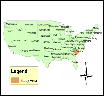 | Figure 1. The Study Area of South Carolina Low Region |
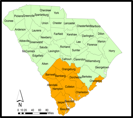 | Figure 1.1. Carolina Low Region |
2.2. Methods
The paper uses temporal-spatial data, agricultural census information and related data based on descriptive statistics and Geographic Information Systems (GIS) to display the trends spatially. The spatial information for the research was obtained from the South Carolina Online data system. This was made possible by the retrieval of spatial data sets of shape and grid files from the South Carolina Department of Health and Environmental Control and the United States Department of Agriculture, (USDA)–National Agricultural Statistics Services (NASS) Geographic Area Data by county in digital form. The statistical output of the variables from the spatial units were mapped and compared across time from 1992 to 2007 and 2010-2012 using ARCVIEW GIS. While the United States Department of Agriculture (USDA) provided farm data for the periods of 1992-2007, Federal geographic identifier codes for the counties were used to geo-code the information contained in the data sets. This information was analysed with basic descriptive statistics, and GIS with particular attention to the temporal-spatial trends at the county level. The relevant procedures consist of two stages.
2.3. Stage 1: Identification of Variables, Data Gathering and Study Design
The first step involves the identification of variables needed to assess degradation in farm landscape and areas adjacent to natural areas. The variables consist of the number of farms, size of farm land and percentages of change. Others are harvested and irrigated crop land, land treated with fertilizer, number of farms using fertilizers and agrochemicals, population, housing elements, market value of building, and goods sold, and others. Additionally, access to databases that are available within the Federal and state archives in South Carolina quickened the search process (See Tables 1-4). The process continued with the design of data matrices for socio-economic and land use (environmental) variables covering the periods from 1992, 1997, 2002, 2007, 2010, 2012 to 2013. The design of spatial data for the GIS analysis required the delineation of county boundary lines. With boundary lines unchanged, a common geographic identifier code was assigned to each of the units to ensure analytical coherency.
2.4. Stage 2: Step 2: Data Analysis and GIS Mapping
In the second stage, descriptive statistics and spatial analysis were employed to transform the original socio-economic and land-use data into relative measures (percentages/ratios). This process generated the parameters for establishing the predictors of degradation and change on the landscape in areas exposed to stress. This was facilitated by measurements and comparisons of the trends over time and space. While this approach allows for change detection, the tables highlight stressors, indicators of degradation, land use patterns and extensive use of resources. The remaining steps involve spatial analysis and output (maps-tables-text) covering the study period, using ARCVIEW 9. With the main spatial units of analysis made up of ten counties in the Carolina Low country. Other components of the geographic data for the study area also covered ecological data of land cover files, paper and digital maps from 1996-2004 as well as 2012.
3. Results
This section presents the results with an initial focus on the analysis of land use variables, the percentage of change and analysis of the trends. This is followed by environmental impact analysis, spatial analysis, the factors and some discussions.
3.1. Temporal Analysis of Land Use
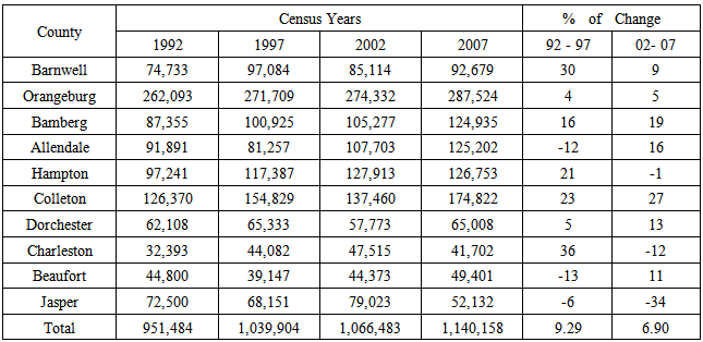
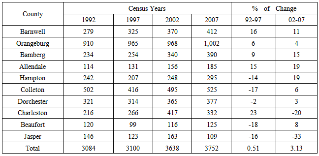
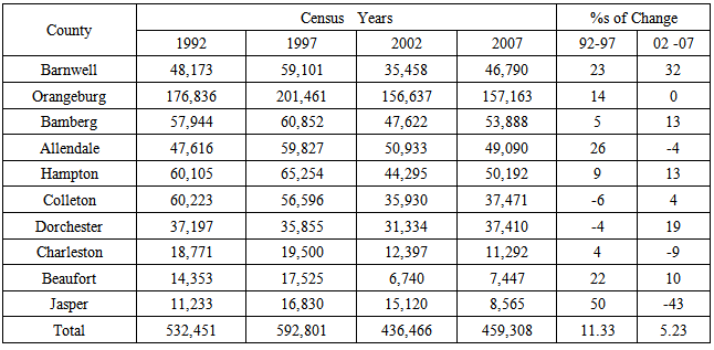
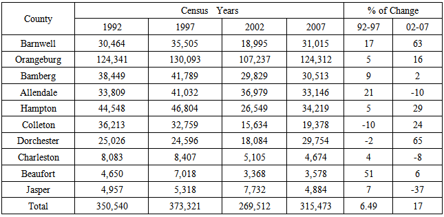
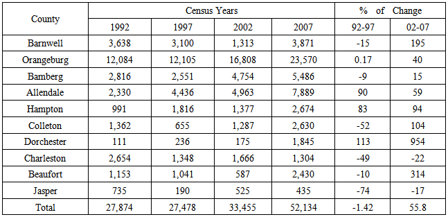
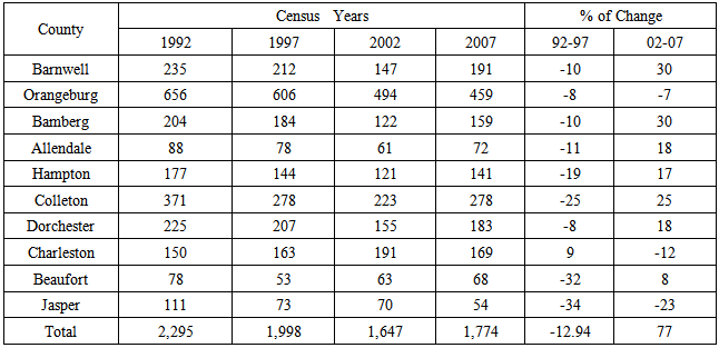
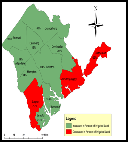
The total size of land in farms of the study area which grew much of the time stood at 951,484 to 1,039,904 in 1992 through 1997 and continued at 1,066,483 and 1,140,158 during the 2002 to 2007 census periods. Of all the counties, four areas (Orangeburg, Bamberg, Allendale, Hampton and Colleton) stood out with bigger farms measuring hundreds of thousands of acres. Among them, Orangeburg not only outpaced the rest of the adjoining areas, but it saw its farm land area soar (from 262,093 to 271,709, and 274,332 to 287,524) between1992-2007. Elsewhere in the same period, Colleton County held on to more land acreages in the order of 126,370, 154,829, 137,460 to 174,822. This is somewhat similar to Hampton where land area stood at 97,241 to 117,387 and 127,913 to 126,753 acres during the four census years. The same can be said of the counties of Bamberg and Allendale which had 87,355-91,891, 100,925 and 81,257 acres between 1992 through 1997. In the ensuing years of 2002 and 2007, the acreages soared from 105,277 to 107,703 and 124,935 -125,202 respectively. Note also that among the other five groups of counties (Barnwell, Dorchester, Charleston, Beaufort, Jasper) with farmland estimated at the tens of thousands, Barnwell, Jasper and Dorchester outpaced all of them. In the case of Barnwell, the acreages ranged from 74,733-97,084 and 85,114 to 92,679 between 1992, 1997, 2002 and 2007 (Table 1).Regarding the available number of farms, regional data showed the South Carolina low country contained 3,084 in 1992, 3,100 in 1997 and 3,638 in 2002 and continued with 3,752 by 2007. The big farm areas of Orangeburg, Colleton, Barnwell and Dorchester emerged with numbers that exceeded the other counties. During that period of 1992, 1997 and 2002, Orangeburg’s initial farm numbers of over 900 jumped to 1,002 by 2007. Next to that comes Colleton county which had over 500-400 farms coupled with Barnwell where the distribution of farms began at 279 followed by the over 324 levels in 1992, 1997 and 2002. In 2007 period, the farm numbers for Barnwell reached 412. Further along the way, Dorchester County not only averaged over 344 farms, but its farm numbers stood at 321, 314, 365 and 377 in the individual censuses. With over 200 farms in the periods of 1992-1997, Charleston’s farm numbers went from 417 to 322 between 2002 through 2007 (Table 2). The total cropland of the low country which grew much of the time stood at 532,451 to 592,801 and 436,466 to 459,308 between 1992 through 2007. The county of Orangeburg with an opening value of 176,836 acres in 1992 saw that number grow to 201,461 by 1997. In the ensuing periods of 2002 -2207, its size of land in crops went from 156,637 to 157,163 acres. In the period of 1992-1997, Hampton County had over 60,000 acres, by the next censuses; the cropland area increased by 44,295-50,192 acres. Elsewhere Colleton county’s land in crops acreages of 60,223 to 56,596 in the initial periods dropped to the over thirty thousand acre mark during 2002-2007. With two other counties Barnwell and Dorchester each with over thirty thousand acres of cropland during the censuses of 1992 -2007, the three counties of Charleston, Beaufort and Jasper rounded up the list of areas with lower cropland acreages during the periods under analysis (Table 3). Over the years, the study area harvested 350,540 to 373,321 acres in the periods of 1992-1997. The intense harvest continued in the ensuing periods of 2002-2007 as crop land area rose from 269,512 to 315, 473 acres. Note the frequency and the high pace of cropland harvest in Orangeburg. In the periods under analysis, the county’s harvested cropland acreages stayed in the order of 124,341, 130,093, 107,237 to 124,312. The other group of counties that were active in harvested cropland such as Bamberg, Hampton, Colleton, Allendale, Barnwell and Dorchester all had sizable acreages areas mostly in the over 20,000 category during the census years. This is higher than the harvested cropland areas for the three remaining areas of Charleston, Beaufort, and Jasper where the size of harvested cropland acreages stood lower during the census periods (Table 4). Irrigated land areas on the other hand, showed notable declines in 6 of the 10 counties in the first census periods of 1992-1992 but soared enormously in the 2002 to 2007 periods (Table 5).
3.2. The Percentages of Change of the Trends
Just as the study area posted back to back percentage gains of 9.29-6.90 in land in farms, four counties in the region (Barnwell, Orangeburg, Bamberg and Colleton) each experienced visible double digit increases. The breakdown of the figures points to 30-36% gains for the counties of Barnwell and Charleston. This was followed by gains of over 20% in the counties of Hampton and Colleton during the census of 1992-1997. While Jasper on the other hand stood out with back to back losses of -6 to -34% between 1992-1997 and 2002-2007, pockets of declines held steady at under -13% for Allendale and Beaufort followed by -1% and 12 percentage declines for Hampton and Charleston during the periods of 1992-2007. Regarding farm numbers, the entire low country not only posted 0.51 to 3.13% gains, but the counties themselves were evenly split in terms of gains and declines between 1992 -1997 (Table 1).Among the counties that experienced declines in the number of farms, Beaufort, Colleton, Jasper and Hampton each posted double digit drops of -18, -17, -16, -14 percentage points followed by the -2% for Dorchester. During the same period, Charleston, Allendale, and Barnwell all made sizable gains of 23, 15, 16 percent while Orangeburg and Bamberg finished with single digits percentage points of 6 to 9. With the exception of the double digit declines of -33 to -20 sustained by Jasper and Charleston, farm numbers grew in other counties. With gains of 143 to 35% in cropland acreages for the entire region between the census periods 1992-2007, only Colleton and Dorchester experienced cropland losses of -6 to -4% while the others posted gains in 1992 and 1997 at the county level (Table 2). Of these counties, Jasper’s cropland area rose by 50% while three other areas Beaufort, Barnwell and Allendale saw increases of over 20%. In the 2002-2007 period, the percentages of change showed drops in three (Allendale -3, Charleston-9 and Japser-43) of the seven counties that finished with similar level of acreages. In the other counties, Barnwell, Bamberg, Hampton, and Dorchester and Beaufort made significant gains of 32 -13 and 19-10 percentage points (Table 3). Given the notable gains of 107-150% in harvested cropland for the study area in the census years of 1992-2007, Barnwell, Orangeburg, Bamberg, Hampton, and Beaufort all posted back to back increases as well. The highest level of gains of over 60 to 20 percentage points occurred in the counties of Beaufort and Allendale in 1992-1997 and in Barnwell, Hampton, Colleton Barnwell and Dorchester. Under the loss column, the counties of Colleton and Dorchester experienced drops of -10 to -2% between 1992-1997 (Table 4). Note also the occurrence of visible declines and strong gains in the land areas devoted to irrigation during the census periods under analysis (Table 5).Table 1. Land In Farms
 |
| |
|
Table 2. Number of Farms
 |
| |
|
Table 3. Total Cropland
 |
| |
|
Table 4. Harvested Cropland
 |
| |
|
Table 5. Irrigated Land
 |
| |
|
3.3. Environmental Impact Analysis
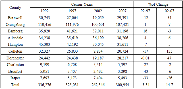
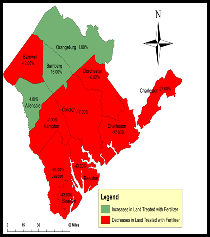
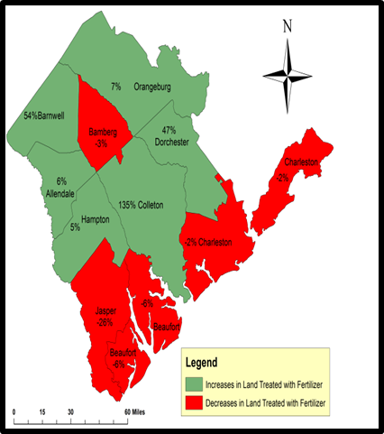
In terms of environmental impact of the trends, the use of fertilizer grew in the area in some periods. In fact during the period in question, fertilizer treatment of land remained sizeable between 2002 through 2007 with mounting threat to the ecosystem. The practice of land treatment with fertilizer reached overwhelming levels considering the vast acreages (326,276- 325,031) covered in the 1992 to 1997 and 262,346-300,954 in the last two censuses. Based on the table, Orangeburg emerged as the area with more lands estimated in the hundreds of thousands treated with chemicals. Land under fertilizer in Orangeburg in 1992 -1997 rose from 110,456- 111,976 acres, and continued at 100,601 to 107,421. The group of counties made up of Barnwell, Bamberg, Allendale, Hampton, and Dorchester each devoted tens of thousands of land to chemical treatment. Among that group, (Hampton, Bamberg, Allendale) fertilizer uses exceeded 40,000 to 30,000 acres in the census periods of 1992 2007. Barnwell on the other opened with 30,743 to 27,064 acres only to rebound by 19,059 to 29,391 acres while Colleton and Dorchester in the 1992-1997 periods used fertilizers on over 20,000 acreages of land. In the last census, land acreages under fertilizer use stood at 8,834 to 20,724 and 19,187 to 28,217 in both counties respectively (Table 6). The use of fertilizer in the study area not only dropped by -118% but it continued in 7 of 10 the counties between 1992-1997 with the only gains of 1.16 and 4 percentage points evident in Orangeburg, Bamberg, and Allendale. In the 2002-2007 periods, when an entirely different trend emerged, fertilized acreages grew by 217% in the low country. During that period, only four counties showed decreases while the applications peaked in 6 others. Amongst the counties, Colleton, Barnwell and Dorchester posted increases of 135%, 54 to 47% in fertilizer use at much higher levels compared to the rest of the study area in the 2002-2007 census years. The same can be said of the number of farms using agrochemicals and fertilizers as shown in Table 6.1. The implication is that being a coastal area and an area highly endowed in marine biodiversity, the run offs from widespread use of chemicals in the area pose enormous threats to the environment and the surrounding ecology. The risks stems from the pace at which fertilizer run offs from agriculture empty into shallow streams and lakes. This often results in a high concentration and elevated toxicity levels of chemicals. There is also the inherent danger to marine life and organisms that depend on the headwaters of the low country for their survival when exposed to dozes of fertilizer nutrients that empty into the waters. Frequent use of fertilizers at that level impedes the carrying capacity of the environment (Table 6). Table 6. Land Treated With Fertilizers
 |
| |
|
Table 6.1. Number of Farms Using Agro-Chemicals and Fertilizers
 |
| |
|
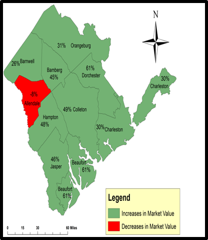
3.4. Spatial Analysis
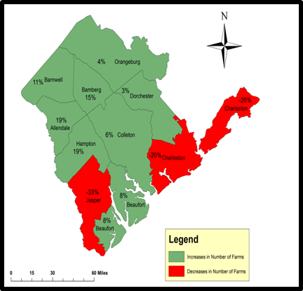
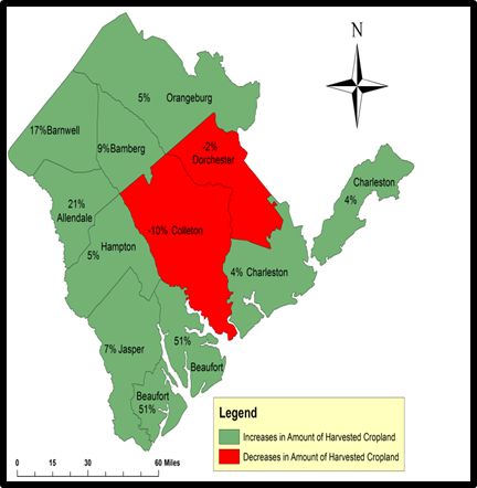
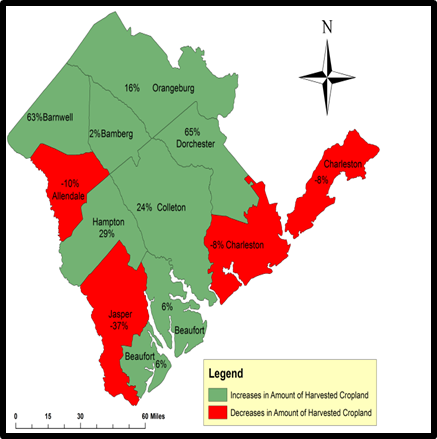
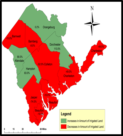
From the analysis, note the large concentration in areas denoted as gaining in farmland (in green) in both the northern and southern part of the study area. Of great importance is that counties like Charleston, Beaufort, and Jasper each moved from gains to loss column as shown in the maps between 1992-1997 and 2002-2007 (Figure 2-2.1). For the number of farms, during the 1992 period much of the gains were concentrated in the upper and lower part of the state with losses evident in the central counties. By the 2002-2007, the study area experienced robust gains (Figure 3-3.1). Notwithstanding the meager declines in space in 2-3 counties during the census periods of 1992-1997 and 2002-2007, harvested cropland soared amazingly during the years with more visible presence (Figure 4-4.1). The same can also be said of land in irrigation in which the counties saw major drops in irrigated land acreage during the first census periods of 1992-1997, until a notable rally with increases in 2002 -2007 (Figure 5-5.1). With extensive declines in the treatment of fertilizers apparent in 1992-1997, note the gradual reemergence of counties in the gains category spread across the low country in 2002 through 2007 (Figure 6-6.1).While gains across counties held steady in the economic variables of market value of goods sold, during the census periods of 1992-1997 with the exception of the declines evidenced in Allendale and Jasper (Figure 7-7.1). The access to government transfer payments offered a contrasting trend which began with an even spread of 5 counties in the declining category and the other 5 dominated by gains. The geographic distribution showed declines in government transfer payments in mostly the northern part and the lower counties of Jasper and Beauport of the study area followed with gains in the middle and south east counties of Charleston, Colleton, Hampton, Dorchester, and Bamberg during the 1992-1997 periods. By 2002 to 2007, most counties (8 of 10) not only experienced gains (turned green) but they all benefited from government assistance through transfer payments. In other words, the increases in government transfer payments were predominant in 80% of the study area with the losses in Jasper and Charleston County (Figure 8-8.1). The population trends between2010 to 2012 on the other hand showed a mix of gains and declines in the respective counties (Figure 9-9.1).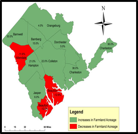 | Figure 2. Farmland Acreage 1992-1997 |
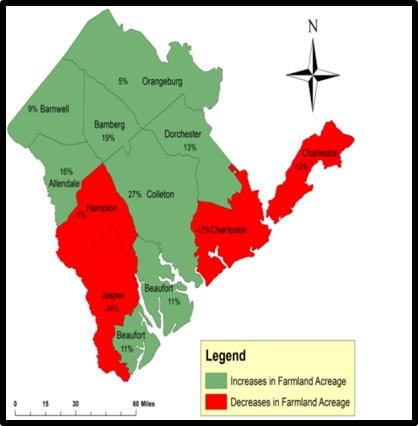 | Figure 2.1. Farmland Acreage 2002-2007 |
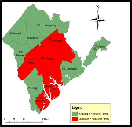 | Figure 3. Number of farms 1992-1997 |
 | Figure 3.1. Number of farms 2002-2007 |
 | Figure 4. Harvested Cropland 1992-1997 |
 | Figure 4.1. Harvested Cropland 2002-2007 |
 | Figure 5. Land Irrigation 1992-1997 |
 | Figure 5.1. Land Irrigation 2002-2007 |
 | Figure 6. Land Treated with Fertilizer 1992-1997 |
 | Figure 6.1. Land Treated with Fertilizer2002-2007 |
 | Figure 7. Market value of Product sold 1992-1997 |
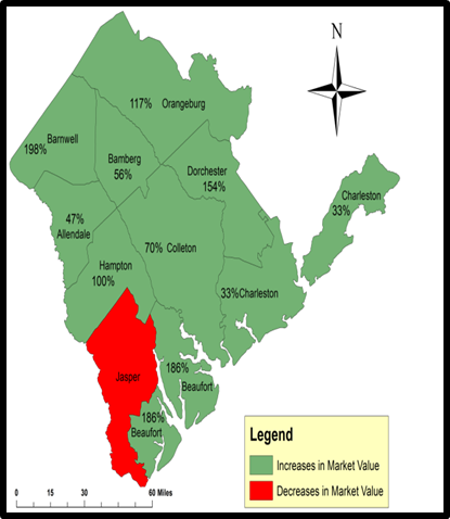 | Figure 7.1. Market value of Product Sold 2002-2007 |
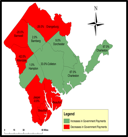 | Figure 8. Government Payments 1992-1997 |
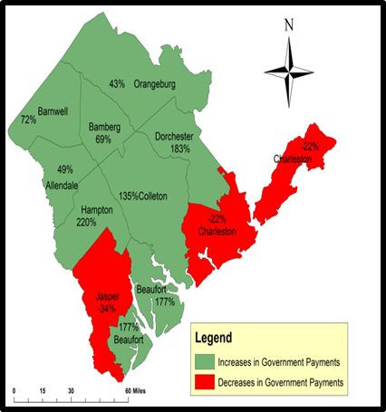 | Figure 8.1. Government Payments 2002-2007 |
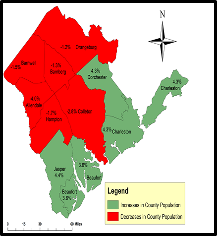 | Figure 9. Population Changes 2010-2012 |
 | Figure 9.1. Population Changes 2010-2013 |
3.5. Factors Responsible For Change
There are several factors shaping farm landscape change in the study area. These factors consist of socio-economic and demographic elements located in the larger agricultural structure of the Low Country.
3.5.1. Economic Elements
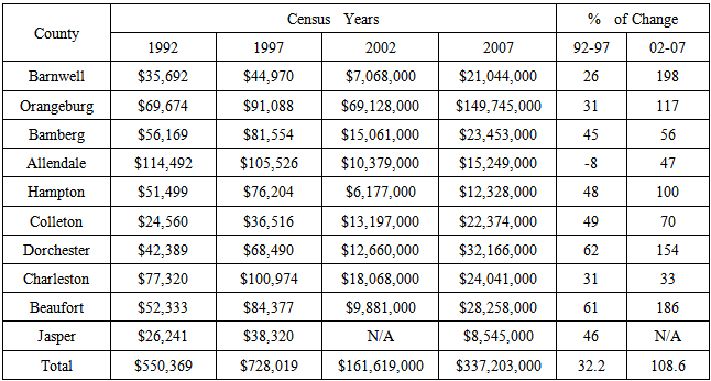
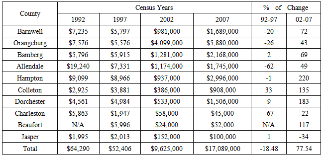
On the economic factors, the market value of goods sold implies a very robust farm sector where cropland and land in farms are actively in use (Table 1.3). The sheer volume of farm trade evident in the area and large commodities in the market place come with sizable incentives and the profits that accrue farming activity. In that setting, farmers in the areas would be inclined into producing more which sometimes results in extensive use of fertilizer nutrients to boost productivity. There is also the problem associated with the economy of scale which often results in consolidation at the expense of smaller farms. Another dimension is the proliferation of government subsidies which reached appreciable levels during the census periods in question. With the eligibility for subsidies sometimes predicated on farm size, less viable farm operations unable to thrive due to the volatility in the market place and falling prices become prone to these pressures and then eventually forced to sell their lands to the largest bidders. This amounts to taking arable land out of operation [20]. Under such a scenario, areas that posted gains in land acreages may have benefited from the rewards of holding on to land in the face of sustained subsides (federal transfer payments) into the low country. In these counties, land acreages in the positive column held steady in some periods hence the gains. During these periods among the economic elements, note that the market value of goods sold and government transfer payments for the study area totaled $550,369, $728,019 and $64,290 to $52,406 in the two census periods. Such outright increases continued with $161,619,000-$337,203,000 by 2002-2007. At the individual county level, in the 1992-1997 period, Orangeburg, Allendale, Bamberg and Charleston sold more goods in the market place with Allendale and Charleston accounting for more dollar values estimated at $114,492 to $105,526, and $77,320 to$100,974. Aside from the $19,240 to $9,099 in money transfer for both Allendale and Hampton, the remainder of the counties Barnwell, Orangeburg, Bamberg and Charleston all took in identical sums of money estimated at over $7000 to 5000 dollar respectively during the 1992-1997 census (Table 7). In the ensuing years of 2002-2007 when Orangeburg county outpaced the others by $69,128,000-$149,745,000 and $4,099,000 to $5,880,000, market value of goods sold and the government transfer payments continued at significant levels in a couple of counties as well (Tables 7 -8). With the overall rates of change of -18.49 to 77.54 in both variables, there came a widespread increase in the market value of goods sold all through 1992-2007. The government transfer payments which decreased earlier on in 1992-1997 rose significantly in the ensuing period of 2002-2007. It is worthy to note that high level gains of 117 to 220 % for the counties of Beaufort, Dorchester, Colleton and Hampton surpassed the rest of the counties in 2002-2007 (Table 8). The volume and magnitude of these transactions as strong indicators of what transpired in the larger agricultural structure may have influenced changes in the farm landscape of the area at the expense of smaller farm holdings that ended up for other uses.
3.5.2. Demography and Housing Development Elements
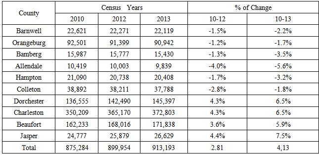
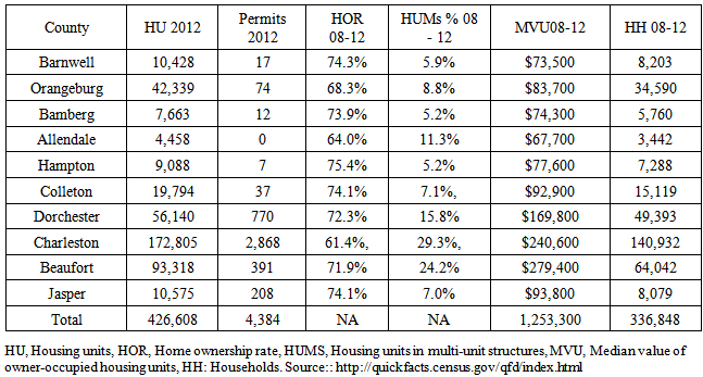
Another dimension to the changing farmland ecosystem is the growing pressure mounted by demographic elements of population and the housing indicators in the study area on the surrounding ecosystem. The interesting thing about the population stems from the high distribution levels of over 800,000 to 913,193 between 2010-2012 and 2013 with much of the large population centers of over 100,000 and more concentrated in mostly Dorchester, Beaufort and Charleston with the latter as the most populated with over 300,000 people between 2010, 2012, and 2013 (Table 9). Like in other counties in the country, serving and maintaining the needs of a timing population of that sort requires the provision of basic infrastructure such as roads, houses and bridges which often come with the issuance of permits approved by panning agencies. The fact that plan approvals and permits are predicated on land use and zoning regulations that are vital for the future development in the area. The provision of infrastructure may have resulted in the conversion of agricultural land areas to housing infrastructure. More so, the pressures from population can be seen from the back to back gains. These changes in population reveal a mix of gains and declines with decreases evident in the low density counties while much of the high population areas posted gains. At the same time, the number of permits in the area among the counties not only stayed sizable, but some of the housing elements such as housing units, average price of homes and percent of households remained higher (Table 10). Monetary benefits from real estate and land speculation that appealed to farmers may have induced farm land owners into selling land for competing land uses hence the resulting declines in the study area.Table 7. Market Value of Goods Sold
 |
| |
|
Table 8. Government Transfer Payments
 |
| |
|
Table 9. Population
 |
| |
|
Table 10. Housing Variables and Factors
 |
| |
|
4. Discussion
From the results of data analysis under a mix scale method of GIS and descriptive statistics, the study area of Carolina Low country experienced changing agricultural landscape at an alarming proportion with impacts on the stability of the surrounding ecology of the area. Being an area rich in biodiversity and natural resources with farming landscapes, between 1992 through 2007, the study area experienced some changes in its acreage of farm land, number of farms, land devoted to cropland and host of other elements located within the larger agricultural sector across time and space. All in all, the combined size of agricultural farmland of the study area which rose consistently at 951,484 to 1,039,904 acres in 1992 through 1997 reached 1,066,483 and 1,140,158 acres in the 2002 to 2007 census periods. Of the counties, four areas most notably (Orangeburg, Bamberg, Allendale, Hampton and Colleton) emerged with bigger farms in hundreds of thousands of acreages. In that group, Orangeburg not only outpaced all the others, but its farm land area soared by 262,093 to 271,709, and 274,332 to 287,524 between1992-2007. Being the most heavily farmed area individually, it dominated in every statistical category in terms of the amount of fertilizer used and the number of farms in the Low country.The environmental analysis of the trends not only showed wide spread treatment of cropland with fertilizer, but the headwaters and marine environment of the area are also at risk from the chemical run offs from agriculture. The changes in the landscapes are attributed to socio-economic elements and demographic elements of population and housing elements from permits, household and the price of homes. Other factors including market value of land to government transfer payment which grew in some of the census periods under analysis and population posted notable variations along with fertilizer use. While preliminary results show gradual declines in farm land and land use elements with slight gains in some years, fertilizer use and the threats of water degradation stayed visible in the region.Essentially, the mix scale analysis based on temporal-spatial techniques of descriptive statistics and GIS, also showed the Low County to be an area of intense farmland activities. This involves the extensive harvesting of land, sizable cropland acreage devoted to agriculture and the irrigation of land to boost farming. With the uncertainties inherent in the weather patterns of the area and the resultant fluctuations in temperature and drought, the Low country remained quite active in irrigation farming. The widespread use of farmland and the pressure put on the cities and counties in that setting to provide infrastructure for a growing population influenced the declines in farmland acreage. This is compounded by rising subsidies and the widespread use of pesticides and the continual threat of the run offs into the surrounding head waters. The implications and benefits of the aforementioned research is that it furnishes planners early warning signals about the state of agricultural land base and exposure to the vulnerabilities induced by human activities. The study affords decision makers the vital clues in pinpointing areas in counties where established thresholds and limits on land use have been exceeded or within manageable levels consistent with the future of development in areas where intense land use is on the rise. Not knowing these scenarios not only results in planners making poor decision, but it puts sustainable management of natural resource assets of the region at risk. Considering the scale of gains and declines in farm land areas and other variables witnessed in the mix-scale analysis of GIS and descriptive statistics. Knowledge of the temporal–spatial distribution of resource abundance and deficits in the low country in general and the ten counties remains highly indispensable in pinpointing critical areas in need of planning. In that setting, areas deemed vulnerable to land resource deficit fall within the threshold of immediate recovery and conservation. The same can also be said of the counties where gains in land base remained frequent and in places where land use is in critical condition or exceeded the suitability thresholds for development and growth. Invoking a suitability clause tag for agricultural land use for such areas could always emerge as a priority among planners in those settings. This may then result in directing development onto preferred areas where infrastructure and other physical amenities are already in place to attract developers hence the benefits for planning. Accordingly, the research also helped showcase the risk associated with widespread use of fertilizers and the need to keep an inventory of its usage, and the vulnerability of headwaters and marine resources. There is also the opportunity to gauge when and how to monitor the trends given the dangers posed by fertilizer run offs to the quality of the surrounding environment. Keeping tab of perverse subsidies of which farmers are entitled to in the form of government transfer payments is also of great importance to policy makers and the beneficiaries. This is essential in gauging the linkages between such policy instruments and landscape change in the low country over the years.In analyzing the geographic dimensions of change and the elements influencing it, the paper used a mix scale method of temporal spatial analysis connected to simple descriptive statistics to GIS. With change attributed to a set of socio-economic variables, GIS mapping points to a gradual spreading of change along with visible dispersal of ecological stressors across time and space in the region. In the absence of existing mitigation efforts, it is evident that the lower South Carolina agricultural landscape is an ecosystem under stress. To remedy the problem, the paper suggests the need for effective land use planning and zoning ordinances, periodic monitoring and assessment of hazards on the landscape followed by a regular use of GIS, the design of a regional information system and a new data infrastructure to optimize access to information.
5. Conclusions
In terms of closure, the results make a substantial contribution to our understanding of GIS assessment of agricultural landscape change research at the regional level. They provide evidence that GIS assessment of the state of farm landscape where farming is prominent are serving as valuable ingredients for new directions in natural resource assessment and the sustainable use of agricultural land. In that setting, studies highlighting the use of a mix scale approach on the Low Country represent new set of ideas shaping our understanding of changing landscape using GIS. The present work corroborates the relevance of regional impact analysis of change and adds new insights on ways of estimating landscape evolution in the Carolina Low country during the 1992 to 2007 census years. Taking a cue from all that, several interesting findings did emerge from the analysis; 1) GIS stood out as an essential tool; 2) Mix scale techniques were quite effective; 3) Farm landscape changed over the years; 4) Widespread risks from rising fertilizer treatment of landscape; 5) Change prompted by several elements. Regarding GIS relevance, it was quite instrumental in visualizing the nature of change. Without such a temporal-spatial framework, decision makers run the risk of prescribing policy change using faulty blueprints at the expense of effective land management and farm retention for communities in the region. Seeing the GIS use in the analysis and the display of changing patterns in particular areas in a landscape. Scrutinizing the geographic dispersion of land use elements coupled with pollutants such as fertilizers and the socio-economic factors of change is vital in managing the farm landscape which is a major economic and ecological asset for citizens. With the extent of change in the area, the timely applications of GIS in that setting is not only indispensable in pinpointing areas impacted by changes in farm landscape, but it provides beneficial uses pertinent to county managers in weighing the indices. Accordingly, GIS technique as used here provides a decision support mechanism for planners in analysing the indices and stressors from landscape change and land suitability in the area. In doing so, this capability conveyed the gravity of change in the study area. With census data becoming available in electronic format and with GIS software now easily accessible, the ability of researchers to conduct advanced spatial analysis in regional landscape assessment has been enhanced. The display of spatial information, including dimensions associated with land use groups, environmental and economic factors, and demographic data in visual form is especially vital due to its potential as a means of communication. For instance, maps are useful in conveying to the reader and land managers which areas in a region are experiencing grave changes where certain factors and conditions associated with declines should be targeted for immediate response. The effective use of appropriate techniques including the GIS and descriptive statistics within a mix scale orientation in this study shows that the present research provided a valuable methodology for the study of regional assessment of farm landscape change. Through the vigorous application of the mix scale approach, the study results clearly indicate that change in land areas had occurred. The development and application of these techniques in the project helped showcase the methodology at the regional level. The exploitation of these techniques in the research along with findings emanating from it, therefore, makes a contribution to our understanding of regional landscape assessment research. These techniques play a fundamental role with regards to the steps upon which regional farm landscape change is built. The project also revealed the utility of the descriptive techniques and GIS in the search for factors associated with change and thus serves as a conduit for future applications in a region. The research unveiled not only the role of mix scale approach as effective model for examining changes in a landscape, but the descriptive statistics component of the model using census data was pivotal in highlighting the snapshots of landscape change.Just as presented in the results, efforts were made to determine the nature of change in the farm landscape as well as the factors responsible for the trend at the region. The measurement of change at the mix scale levels based on a snapshot of the various levels is an improvement to the previous efforts when this study was initiated. Considering that the farm landscape of the region underwent changes of gains and declines, it is obvious that there are a growing number of variations in the farmland index that regional planners are unaware of. If the managers and planners had an adequate monitoring mechanism in place during periods of change, they would have been able to keep the dwindling land base under control. This is attributable to the absence of an index for gauging stability and threats to land. By showing such indices for the purposes of aiding monitoring and directing development to suitable areas, the study did fill a void in a relevant area. This allows for a quick appraisal in the display of declines and gains in farmland acreages. In critical situations, such an approach affords land managers a framework for promoting conservation activities which encourages preservation of the land base and best management practices. Being the pathway for measuring change, the findings outlined herein serves the needs of planners in weighing the significance of emerging patterns and their impacts on the local community. Keeping decision makers abreast of change patterns in this manner enhances their ability to track competing uses and to conduct appraisals as to whether current land use practices are suitable and in conformity with restrictions limiting use around farm operations.In pinpointing the growing use of fertilizer on the landscape in an area rich in biodiversity and abundance of freshwater, the findings not only stand as a timely piece of work but a major step in indicating the dangers of pollution threats in areas adjacent to the head waters of the region. Knowing the risks of spatial dispersal of such stressors, would benefit regulators in the crafting and monitoring of quality standards for the head waters. In the absence of such benefits, regulators will face uphill battles in mitigating ecosystem strain on the landscape. Considering that various factors associated with the use of farmland in the study area were not estimated previously, the role of these factors in impeding landscape gain merits prompt attention from the government entities charged with the task of safeguarding open spaces and land assets using the index developed herein. In light of this, this study not only finds a practical use, but the measurement of various dimensions of change in the farm landscape that had not been detected before in the area could emerge as a priority for managers. The ability of this project to unveil elements behind declines and gains in the landscape shows regional assessment can serve as a viable tool for promoting sustainable land management. The analysis of links between landscape declines and factors known to fuel degradation is evidence of the study’s promise in helping identify predictors of change and degradation.The significance of the result herein presented raises several questions for further scholarship and decision making that would need to be answered in the region and they include: what will the changing landscape be like in the coming years? What will be the core enablers of this change? What form will the geographic dimensions of the landscape evolution assume? Which areas will be suitable for farming? Because of their significance to many aspects of future plans and communities in the region, decision makers must grapple with how to integrate answers to these questions in their long range plans in the coming years before it is too late. In that light, current studies can always build on the analysis herein using these questions as a template to further research on farm landscape change with focus on how change impacts the livelihood of communities by limiting access and sustainable use of the land base. The benefit is that it offers a set of parameters upon which managers can draw from as they craft measures best suited for their counties in order to ensure continued access to farm landscape and sustainable use. In so doing, land managers can become cognizant of issues arising they would not have known in the areas under their jurisdiction thanks to this research.
References
| [1] | Merem, E.C. (2014 March). Assessing Agricultural Landscape Change In Northern Mississippi. World Environments. 4:2:43-60. |
| [2] | Merem, E.C., & Wesley, J.M. (2014). GIS Analysis of Environmental Issues In Lower Savannah Watershed. Proceedings of the 24th Annual AEHS Conference, San Diego: California. March 17-20 2014. |
| [3] | Merem, E.C., & Wesley, J.M. (2014). “GIS Assessment of the Ecological Impacts of Farm Landscape Change in South Carolina Lower Region” Proceedings of the National Water Quality Association Conference NWAQC, Cincinnati: Ohio, April 28- May 2 2014. |
| [4] | Merem, E.C., & Wesley, J.M. (2013). “GIS Analysis of Shifting Farm landscape in Northern Louisiana Region” Proceedings of the 10th International Symposium On the Recent Advances in Environmental Health, Jackson: MS, September 2013. |
| [5] | Merem, E.C. (2013 January). Geospatial Assessment of The Impacts of Changing Agricultural Landscape In Louisiana. The Journal of Marine Sciences, 3:19-29. |
| [6] | Merem, E.C. (2014 March). The Analysis of Coal Mining Impact On West Virginia’s Environment. British Journal of Applied Science and Technology, 4:8:1171-1197. |
| [7] | Merem, E.C. (2012 September). Using Geospatial Information Systems in Assessing Water Quality In The Mid Atlantic Region Agricultural Watershed of Maryland. The International Journal of Ecosystem. 2:5: 112-139. |
| [8] | Merem, E.C., & Twumasi, Y.A. (2011 June 23rd). The Applications of GIS in the Analysis of the Impacts of Human Activities on South Texas Watersheds International Journal of Environmental Research and Public Health. 8:6: 2418-2446. |
| [9] | Merem, E.C., & Twumasi, Y.A. (2012). Using GIS To Assess the Contributions of Farming Activities to Climate Change In The State of Mississippi. The British Journal of Environment and Climate Change. 2:2.1-15. |
| [10] | Merem, E.C., & Wesley, J.M. (2013). Analyzing the Changing Agricultural Landscape of Northern Louisiana Using GIS. Proceedings of the AEHS Conference, Sandiego: California March 2013. |
| [11] | United States Department of Agriculture. (2012). Various Years Census Data: County Highlights. Washington, D.C: USDA- NASS. |
| [12] | United States Bureau of Census (2013): Census Quick Facts. Washington, D.C: Bureau of Census. |
| [13] | United States Environmental Protection Agency (1989). South Carolina Superfund Site: Savannah River Site. D.C: Washington. US EPA. |
| [14] | Conservation Voters of South Carolina. (2014). Issues Public Health: A Clean Environment is Our Right. Columbia, SC: Conservation Voters of South Carolina, 1-2. |
| [15] | Conservation Voters of South Carolina. (2014). Issues Abundant Waters: Our Savings In The Bank. Columbia, SC::Conservation Voters of South Carolina. 1-2. |
| [16] | South Carolina Department of Health and Environmental Control. (2010). The South Carolina Mercury Assessment and Reduction Initiative 2010. Retrieved on March 25th 2014 Fromhttps://www.sedhec.gov./environment/admin/mercury/htm/mercurysc.htm. |
| [17] | South Carolina Department of Health and Environmental Control (2014). Healthy People Living In Healthy Communities. Retrieved on March 25th 2014 From http://www.scdhec.gov/adminsitration/hplhc/environmrent.htm. |
| [18] | South Carolina Department of Health and Environmental Control. (2014). Coastal Hazards: Ocean and Coastal Resource Management. Retrieved on March 25 2014 From https://www.scdhec.gov/environment/ocrm/coastal_hazzards.htm. |
| [19] | South Carolina Department of Health and Environmental Control. (2014). Critical Area and Wetland Permitting Retrieved on March 25th 2014 Fromhttps//www.scdhec.gov/environment/ocrm/permit_critical _area.htm. |
| [20] | McReynolds, R. (2014), Backroom Dealing On Farm Bill. Carolina Farm Stewardship Association. Retrieved on March 25th 2014 Fromhttp://www.crolinafarmstewards.org/backroom-dealing-on-farm-bill. |
 Abstract
 Reference
 Full-Text PDF
 Full-text HTML