1. Introduction

Accounting for a fifth of humanity’s food, wheat is second only to rice as a source of calories in the diets of consumers in the developing countries. It is the first source of protein (Braun et al., 2010). Wheat is an especially critical “stuff of life” for approximately 1.2 billion “wheat dependent” and 2.5 billion “wheat consuming” poor men, women and children who live on less than USD 2 per day; and for approximately 30 million poor wheat producers and their families (CIMMYT, 2012).

If population growth continues at double the growth of wheat production, there will likely be serious difficulties in maintaining wheat food supply for future generations (Dixon et al., 2009; CIMMYT, 2012). In 2010, African countries spent more than US$ 12.5 billion on importing 32 million tons of wheat. Demand for wheat in Africa is growing faster than for any other food crops. Demand for wheat in the developing world is expected to increase by 60% by 2050 (Rosegrant and Agcaoili, 2010; CIMMYT, 2012). The challenges of globally low and fluctuating wheat production, rising consumer demand and higher food prices require efforts that dramatically boost farm-level wheat productivity and reduce global supply fluctuations. Productivity growth is considered to be one of the long term solutions to these challenges (Diao et al., 2008).

In Ethiopia, the major challenges facing agriculture are low productivity, low use of improved farm inputs, and dependency on traditional farming and rainfall. As a result, food insecurity and poverty are prevalent in the country. Wheat is one of the major food crops with low productivity. It is the second important cereal crop with annual production of about 3.43 million tons cultivated on area of 1.63 million hectares (CSA, 2013). It occupied about 17% of the total cereal area with average national yield of 21.10 q/ha. This is the lowest yield compared to the world average of 40 q/ha (FAO, 2009). The low yield has made the country unable to meet the high demand and the country remains net importer despite its good potential for wheat production (Rashid, 2010). Increasing yield and meeting the high demand has become the main concern of government’s agricultural policy and extension activities.

Agricultural extension activities have been concerned with the promotion, adoption and scaling up of wheat row planting practices; and adoption of the practice is seen as the factor for wheat yield enhancement in the country. As a result, manual planting of wheat in row has become one of the agronomic practices of smallholder farmers in the country. The conventional planting method, that is broadcasting seed by hand at high seed rates, reduce yield because uneven distribution of the seeds makes hand weeding and hoeing difficult, and plant competition with weeds lowers wheat growth and tillering. This causes wheat yield reduction. However, row planting with proper distance between rows and plant density allows for sufficient aeration, moisture, sunlight and nutrient availability leading to proper root system development.

Though the impact of row planting method is linked to problems in implementation of the program and its recommendations, methodological issues, and over optimism of the potential of row planting in real farm setting (Vandercasteelen et al., 2013), the row planting technique is seen as good agronomic practice by agricultural policy makers and extension personnel. However, there is lack of empirical study on the impact of wheat row planting on wheat yield of smallholders. Therefore, the main objective of this study was to evaluate the impact of manual wheat row planting on wheat yield of smallholders. The result of the study helps to formulate proper extension activities in the promotion and scaling up good agronomic practices in highland and lowland wheat producing areas of the country.

2. Research Methodology

2.1. The Study Area

The study area, Arsi Zone, is found in the central part of the Oromia National Regional State of Ethiopia. The zone astronomically lies between 7° 08’ 58’’ N to 8° 49’ 00’’ N latitude and 38° 41’ 55’’ E to 40° 43’ 56’’ E longitude. The area is divided into five agro-climatic zones mainly due to variation in altitude. It is dominantly characterized by moderately cool (about 40 percent) followed by cool (about 34 percent) annual temperature. The mean annual temperature of the Zone is found between 20-25℃ in the low land and 10-15℃ in the central high land.

On average, the zone gets a monthly mean rainfall of 85 mm and an annual mean rainfall of 1020 mm. The area receives well distributed rainfall both in amount and season. This characteristics makes the zone good potential for production of various agricultural crops. Wheat is a major crop and it accounts for 42% of the total cereal area cultivated in the study area, with total output of 5.12 million quintals from 0.21 million hectares of cultivated land (CSA, 2013). These characteristics make the zone the first potential area for wheat production in the country.

2.2. Sampling Techniques

The study used three stages probability sampling procedures for sample selection. In the first stage, lists of major wheat producing highland and lowland districts were prepared. The criteria for inclusion in the list include high potential for wheat production both at regional and national perspectives, availability of research and extension intervention programs embracing wheat producers in the districts, and distribution of newly released improved wheat varieties as well as adoption of wheat row planting practices. From separate lists of highland and lowland districts, one district was randomly selected from each agro-ecology (highland and lowland). The selected districts were, namely, Lemu-Bilbilo from the highland and Dodota from the lowland districts.

In the second stage of the probability sampling, a list of major wheat growing lower administrative divisions (kebeles) in which wheat row planting has been practiced was prepared. Taking in to account the resources available, two kebeles were selected from each district with simple random sampling. In the final stage, a list of wheat households was prepared for each selected kebele. Sample households were selected by simple random sampling. The sample size was determined based on the formula given by Krejice and Morgan (1970), and allocation of sample size to each district and kebele was made proportionate to the size of wheat farm households’ population of each district and kebele. Accordingly, from a total of randomly selected 248 sample size, 165 households were selected from the highland district (Lemu-Bilbilo) and 83 households were selected from the lowland (Dodota) district. From the selected households, 40 and 41 percents were participant households in wheat row planting in Lemu-Bilbilo and Dodota districts, respectively in 2012/13 cropping season i.e. during the survey season.

2.3. Data Collection

The data for study was collected from both primary and secondary sources. Cross-sectional data was collected from the survey of randomly selected sample farmers. For the primary data collection, specifically designed and pre-tested questionnaire based on the objective of the study, and trained data enumerators was used. Both quantitative and qualitative information were collected. The data collection included households’ demographic and socioeconomic characteristics (family sizes, age and sex structures, education, etc), land holding (agricultural, grazing, wheat land, and others), farm inputs utilization (seeds, fertilizers, herbicides and fungicides, labor utilization, credit, extension services), farm outputs, input and output prices, agronomic practices including crop rotation, wheat row planting and its inputs and output, etc. Secondary information on rainfall amounts (annual mean and cropping season), temperature, etc were also collected. The survey was carried out in the months of May and June 2013.

2.4. Analytical Methods

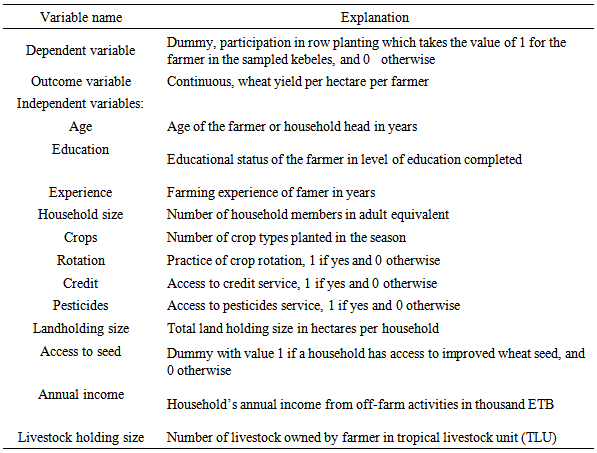
Participation in wheat row planting cannot be random. Propensity score matching (PSM) relaxes randomization when compared to parametric models; and its simplicity in relaxing the assumptions of functional forms that are imposed by parametric regression models makes it the preferred technique in impact evaluation. Rosenbaum and Rubin (1983) have developed the PSM statistical tool, and since then the technique has attracted attention of social and economic program evaluators. In this study, propensity score matching was used in order to capture the impact of planting of wheat in row on yield of wheat. The matching technique is widely used in impact evaluation in the absence of baseline data and when randomization is very unlikely. PSM allows the estimation of mean impacts without arbitrary assumptions about functional forms and error distributions. Furthermore, despite that regression models use full sample, PSM is confined to matched one (i.e., the region of common support). Therefore, impact estimated with parametric models (i.e., based on full or unmatched samples) are more biased and less robust to miss-specification of regression functions than those based on matched samples (Ravallion, 2005).

The PSM method can be used in many fields of social sciences to evaluate the effects of public program and policies (Janan and Ravallion, 2003). The technique enables us to extract from the sample of non-adopters (non-participating) households a set of matching households that look like the adopters (participating) households in all relevant pre-intervention characteristics. In other words, PSM matches each adopter household with a non-adopter household that has (almost) the same likelihood of adopting row planting. The aim of matching is to find the closest comparison group from a sample of nonparticipants to the sample of program participants. "Closest" is measured in terms of observable characteristics. Individuals with similar propensity scores are paired and the average treatment effect is then estimated by the differences in outcomes (Greene, 2012).

In this study, the main pillars of PSM were wheat farmers, the treatment (participant farmers in wheat row planting) and potential outcome (wheat yield). The idea was to match those wheat farmers that practice wheat row planting with that of a control group (non adopters of row planting) sharing similar observable characteristics. Then mean effect of wheat row planting was calculated as the average difference in yield between adopters (participant in row planting) and non adopter (non participant in row planting) groups i.e. the impact was the change in wheat yield as an outcome indicator. The use of propensity score matching model was to answer the question “what would be wheat output per hectare for farmers who planted wheat in-row had these farmers not practiced planting wheat in-row?”

Participant and non participant farmers in wheat row planting were matched exactly on farmer characteristics (age, education, farming experience, land holding size, number of crop types planted in the season, practice of crop rotation, access to credit services and improved wheat seed, household size, livestock holding size, and off-farm income). These variables were used to select comparison farmers via different matching estimators; namely, nearest neighbor matching, caliper and kernel.

Logistic regression (logit model) was fitted using method of planting as dependent variable, the set of farmers’ socioeconomic characteristics as explanatory variables which were assumed to determine practice of wheat row planting and the outcome variable, wheat yield. Table 1 gives definitions of the variable used in the PSM.

Table 1. Definitions of variables in propensity score matching

Based on Rosenbaum and Rubin (1983), propensity score can be defined as the conditional probability of receiving a treatment given pretreatment characteristics. Therefore, Let Y_i^T and Y_i^C are the outcome variable for participant (row planting) and non-participant (broadcast), respectively. The difference in outcome between treated and control groups can be seen from the following mathematical equation:

(1)

Y_i^T: Outcome of treatment (wheat yield in quintal per hectare of the i^th household, when he/she is participant),

Y_i^C: Outcome of the non-participant individuals (i.e wheat yield of the i^th household when he/she is non participant in wheat row planting), Δ_I is change in the outcome as a result of wheat row planting for the i^th household. Let the above equation be expressed in causal effect notational form, by assigning D_i=1 as a treatment variable taking the value 1 if the individual received the treatment (row planting) and 0 otherwise. Then the Average Treatment Effect of an individual i can be written as:

(2)

Where ATE, Average Treatment Effect, which is the effect of treatment on the outcome variable:

E(Y_i^TD_i=1): Average outcomes for individual, with treatment, if he/she would participant (D_i=1).

E(Y_i^cD_i=0): Average outcome of untreated, when he/she would non-participant, or absence of treatment (D_i=0). The Average Effect of Treatment on the Treated (ATT) for the sample households is given by:

(3)

The fundamental evaluation problem in estimation of impact is that it is impossible to observe a person’s outcome for with and without treatment at the same time. While the post-intervention outcome E (Y_i^TD_i=1) is possible to observe, however, the counterfactual outcome of the i^th household when she/he does not use the treatment is not observable in the data.

Thus, estimation of ATE can give a seriously biased result, due to the fact that the population can differ among the comparison group, not only in terms of treatment status, but even in terms of other characteristics: this problem is often referred to as the “fundamental problem of causal inference’’. Thus, simple mean comparison between the treated and non-treated can be misleading, yet taking the mean outcome of non-participants as an approximation is not advisable, since participants and non-participants usually differ even in the absence of treatment (Caliendo and Kopeinig, 2008). A solution to this problem is to construct the unobserved outcome which is called the counterfactual outcome that households would have experienced, on average, had they not participated (Rosenbaum and Rubin, 1983), and this is the central idea of matching.

According to Rosenbaum and Rubin (1983), the effectiveness of matching estimators as a feasible estimator for impact evaluation depends on two fundamental assumptions, namely:

Assumption 1: Conditional Independence Assumption (CIA): It states that treatment assignment (D_i) conditional on attributes, X is independent of the post program outcome (Y_i^T,Y_i^C). In formal notation, this assumption corresponds to:

(4)

This assumption imposes a restriction that choosing to participate in a program is purely random for similar individuals. As a consequence, this assumption excludes the familiar dependence between outcomes and participation that lead to a self selection problem (Heckman et al., 1998).

The conditional average effect of treatment on the treated has a problem, if the number of the set of conditioning variables (X’s) is high, and thus the degree of complexity for finding identical households both from program users and non-users becomes difficult. To reduce the dimensionality problem in computing the conditional expectation, Rosenbaum and Rubin (1983) showed that instead of matching on the base of X’s one can equivalently match treated and control units on the basis of the “propensity score” defined as the conditional probability of receiving the treatment given the values of X’s, notationally expressed as P(X_i)=Pr(D_i=1X_i)

Where Pr is the probability or the logistic cumulative distribution, D_i = 1 if the subject was treated, X_i is a vector of pre-treatment characteristics.

In estimating the propensity scores, all variables that simultaneously affect participation in the program and outcome variables were included. Thus, the average treatment effect on the treated conditional on propensity score P(X) can then be written as:

(5)

Assumption 2: Assumption of common support:

(6)

The assumption is that P(x) lies between 0 and 1. This restriction implies that the test of the balancing property is performed only on the observations whose propensity score belongs to the common support region of the propensity score of treated and control groups (Becker and Ichino, 2002). Individuals that fall outside the common support region would be excluded in the treatment effect estimation. This is an important condition to guarantee improving the quality of the matching used to estimate the ATT. Moreover, implementing the common support condition ensures that a person with the same X values (explanatory variables) have a positive probability of being both participant and non participants (Heckman et al., 1999). This implies that a match may not be found for every individual sample. Rosenbaum and Rubin (1983) describe assumption one and two together as strong ignore-ability assumption.

According to Caliendo and Kopeinig (2008), there are steps in implementing PSM. These are estimation of the propensity scores, choosing a matching algorithm, checking the common support condition, and testing the matching quality. Finally, logistic regression (logit model) was fitted using method of planting as dependent variable, the listed socioeconomic variables as explanatory variables which were assumed to determine practice of wheat row planting and the outcome variable, yield.

3. Results

3.1. Descriptive Results

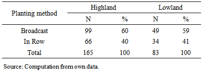
The number of sample households who practiced planting wheat in row was 40 and 41 percents while those who used the conventional planting method (broadcast) comprise 60 and 59 percents of sample households in highland and lowland districts, respectively (Table 2). The proportion of participant farmers in wheat row planting was almost equal in the two areas.

Table 2. Sample farmers' wheat planting methods

Table 3 displays average yield of row planting and broadcast methods. Average yield of row planting was 27.95 q/ha in the highland district and 17.37 q/ha in the lowland district. The average yield of broadcast planting method was 23.35 q/ha and 15.74 q/ha in the highland and lowland, respectively. This shows that the average yield of wheat row planting was higher than the broadcast planting method in both areas. The average percentage yield gain from row planting was 19.7 and 10.31 percents in the highland and lowland, respectively (Table 3). The t-test for the mean yield difference between the two planting methods gave significant t- statistic in the highland and non significant t-statistic in the low land, depicting that the mean yield difference between the two planting methods was significant in the highland, and non significant in the lowland district at 1% level of significance. Similarly, the t-test for mean wheat yield difference between the two districts shows significant t-value (t-value = -10.5795, p-value = 0.0000), indicating significant wheat yield difference between the highland and lowland districts. The test for mean yield difference by methods of planting between the two districts also gives statistically significant difference at 1% level of significance (t-value = -3.7602, p-value = 0.0002).

Table 3. Average wheat yield of planting methods (q/ha)

3.2. PSM Estimation Results

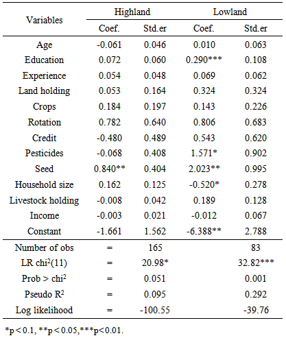
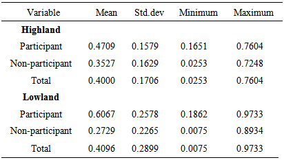
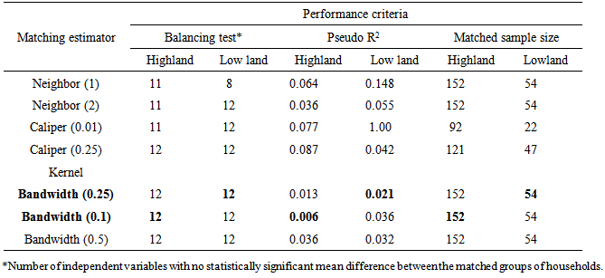
Using logit model, equations (1) to (6) and the variables listed in Table 1, Propensity Score Matching (PSM) analysis for the impact of row plating on wheat yield was conducted using psmatch2 command and STATA version 11 software program. The logit regression of propensity score (Table 4) depicts that the conditional probability of participation in wheat row planting was affected by educational level of household head, access to pesticides and improved seed, and household size in the lowland district whereas access to improved seed was the significant factor that affected the conditional probability of participation in wheat row planting. It shows that education and access to farm inputs especially improved wheat seed increase the probability of participation in wheat row planting. Some variables negatively influenced the conditional probability of participation in row plating. For instance, in the highland district, age of household head, access to credit and pesticides services, livestock holding size and off-farm income negatively affected probability of participation in row planting. In the lowland district, household size and off-farm income negatively affected probability of participation in wheat row planting. It seems that households with access to credit, off-farm income and more livestock holding size are not willing to use time and labor consuming manual wheat row planting practice. The overall effect of the independent variables on probability of participation was different from zero as implied by significant chi-square statistic of the likelihood ratio test in the two districts. However, it has to be noted that the success of propensity score estimation is assessed by the resultant balance rather than by the fit of the models used to create the estimated propensity scores (Dehejia and Wahba, 2002).

Table 4. Logit estimate for propensity score for study districts

Matching of participant and nonparticipant households was carried out to determine the common support region. The basic criterion for determining the common support region is to delete all observations whose propensity score is smaller than the minimum propensity scores of participants and larger than the maximum in the control group (Caliendo and Kopeining, 2008). That is, deleting all observations out of the overlapping region.

Table 5 shows the distribution of propensity scores of both participant and non participant households of highland and lowland districts before common support condition is imposed. The table shows that there is wide area in which propensity score of participant and non participant households are similar. Therefore, it is possible to match the two groups using the common support region or overlapping area of propensity scores.

Table 5. Summary of propensity scores for sample farmers

The summary statistics of propensity scores of farmers (Table 5) depicts that the common support region lies within the range of 0.1651 to 0.7248 propensity scores for both participant and non participant households in the highland district. In the lowland, the propensity scores (the conditional treatment probability) range from 0.1862 to 0.9733 for participant households, and 0.0075 to 0.8934 for non participant households. Therefore, the propensity scores for the common support region (overlapping region) range from 0.1862 to 0.8934 (Table 5).

Choice of matching algorithm was carried out from nearest neighbor, caliper and kernel methods. The choice of estimator based on three criteria; namely, balancing test, pseudo R² and matched sample size. The matching estimator which balances more independent variables, has low pseudo R² value and results in large matched sample was chosen as being the best estimator of the data. Accordingly, Kernel matching method with bandwidth of 0.1 was found to be the best estimator of the data of highland district (Table 6). As depicted in the table, relatively, this estimator resulted in least pseudo R² (0.006) and large number of matched sample size (152) by discarding 13 unmatched households from total of 165 households. Similarly, Kernel matching with bandwidth 0.25 was found to be the best estimator for data of lowland district. It resulted in lowest pseudo R² value, well balanced covariates, and large sample size by discarding 29 unmatched households from the sample of lowland district.

Table 6. Performance of matching estimators for sample farmers

The impact of wheat row planting on household’s wheat yield was based on sample of matched treated and control groups. The estimated average treatment effect (ATT) for highland district showed that wheat row planting has significant effect on yield of participant farmers with significant t-statistic (3.79) at 1 percent significance level (p < 0.01). The average wheat yield of participant households in wheat row planting was higher by 13.9 percent when compared with the average yield of non participant households in the highland district. However, in the lowland district, the average row planting effect (ATT) estimation result showed that wheat row planting was not associated with increased wheat yield as indicated by statistically not significant t-value (Table 7). The average wheat yield of participant households was higher than that of non participant households by 0.3 percent with t-value of 0.02, implying statistically non significant yield difference between participant and non participant households in wheat row planting in the lowland district. This implies that the biophysical conditions and other agronomic practices may have more impact on wheat yield than the row planting in the lowland agro-ecology.

Table 7. Estimate of average treatment effects for the study districts

Though, there is lack of empirical knowledge on the impact of manual wheat row planting on yield in the country, the result is more or less consistent with what has been found by Vandercasteelen et al. (2013) on the study of promotion of tef row planting on farmers’ yield in Ethiopia. The result of this study helps to weigh the yield advantage of the labor intensive farming practice (manual wheat row planting) in enhancing wheat yield and economic benefit, and redirect the use of scarce farm inputs to more productive agricultural practices.

4. Conclusions

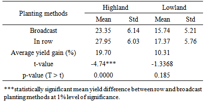
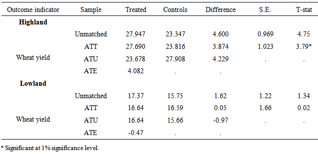
The objective of this study was to evaluate the impact of manual wheat row planting on yield of smallholder farmers in selected highland and lowland districts of Ethiopia. Propensity score matching (PSM), binary logit, and cross-sectional survey data were used to attain the objective of the study. Data on farmers’ inputs and output, household socioeconomic characteristics, access to and use of various farm inputs, use of improved agronomic practices’, etc were collected from randomly selected 248 households (165 from highland and 83 from lowland districts) for 2012/13 cropping season. The analyses of the data resulted in significant yield impact on wheat yield of those farmers who participated in wheat row planting when compared to farmers that used the conventional broadcast planting method in the highland. The mean yield of row planted wheat was higher by 13.9 percent when compared to the mean yield of broadcast planting method. This shows that wheat row planting has significant effect on wheat yield of farmers in the highland area. However, the impact of wheat row planting on yield in the lowland district was statistically non significant, implying that row planting in the lowland did not result in statistically significant yield advantage.

However, placing wheat seed in-row alone might have not been factor for yield advantage over broadcast planting method. Other agronomic practices such as row and seed spacings, seed and fertilizer rates, early hand weeding and hoeing as well as other agronomic and management practices need to be considered for increased wheat yield in the study area. Therefore, the study recommends that agricultural research and extension activities need to consider additional agronomic practices along with the row planting method in order to increase wheat yield, and for the successful promotion, adoption and scaling up of good agronomic practices.

ACKNOWLEDGEMENTS

We are highly grateful to Ethiopian Institute of Agricultural Research (EIAR) and East African Agricultural Productivity Project (EAAPP) for their financial and material support for conducting field survey for data collection. Many thanks go to data enumerators for their painstaking involvement in data collection for the study.