-
Paper Information
- Next Paper
- Previous Paper
- Paper Submission
-
Journal Information
- About This Journal
- Editorial Board
- Current Issue
- Archive
- Author Guidelines
- Contact Us
International Journal of Agriculture and Forestry
p-ISSN: 2165-882X e-ISSN: 2165-8846
2013; 3(4): 145-151
doi:10.5923/j.ijaf.20130304.04
Measuring the Resemblance in Weight of Two Group of Broiler Birds Using the Mantel Test Analysis
 Abstract
 Reference
 Full-Text PDF
 Full-text HTML
Aronu C. O.1, Ogbogbo G. O.2, Bilesanmi A. O.1
1Department of statistics Nnamdi Azikiwe University, Awka, Nigeria
2Department of statistics Delta State Polytechnic, Oghara, Nigeria
Correspondence to: Aronu C. O., Department of statistics Nnamdi Azikiwe University, Awka, Nigeria.
| Email: |  |
Copyright © 2012 Scientific & Academic Publishing. All Rights Reserved.
Feeding in broiler production is viewed as the major component in determining the weight and profitability of broiler birds. The choice of feed type is often dependent on the target of the farmer; since it is believed that broilers require energy for growth of tissue, maintenance and activity which varieties of feed types may or may not have the ability to provide such nutritious value. The Mantel test analysis was used to measure the linear resemblance in weight of two groups of broiler birds feed with two feed type. Secondary data obtained from the records department of Ekeukwu Farms Anambra state – Nigeria for a period of eight weeks. Where sixty broiler birds were divided into two groups, one labelled group A was feed with the first feed while group B was feed with another type of feed. The weights of the birds were recorded weekly for the period of eight weeks. It was observed that there exist a week positive resemblance between the weight of Group A broiler birds and Group B broiler birds with an association of 35.72% and a P-value of 0.0002 which fall’s on the rejection region with a significance level of 5% (α = 0.05).
Keywords: Distance Matrices, Hypothesis, Linear Independent, Monotonic, P-value, Resemblance
Cite this paper: Aronu C. O., Ogbogbo G. O., Bilesanmi A. O., Measuring the Resemblance in Weight of Two Group of Broiler Birds Using the Mantel Test Analysis, International Journal of Agriculture and Forestry, Vol. 3 No. 4, 2013, pp. 145-151. doi: 10.5923/j.ijaf.20130304.04.
Article Outline
1. Introduction
- One of the key determining factors for a positive economic broiler production is fast growth rate and efficient feeding strategy. Feeding in broiler production is viewed as the major component in determining the weight and profitability of broiler birds. To support optimum performance, broiler rations must be formulated to give the correct balance of energy, protein and amino acids, minerals, vitamins and essential fatty acids. The choice of feed type is often dependent on the target of the farmer; since it is believed that broilers require energy for growth of tissue, maintenance and activity which varieties of feed types may or may not have the ability to provide such nutritious value. Carbohydrate sources, such as corn and wheat, and various fats or oils are the major source of energy in poultry feeds. Feed proteins, such as those in cereals and soybean meal, are complex compounds which are broken down by digestion into amino acids. These amino acids are absorbed and assembled into body proteins which are used in the construction of body tissue, for instance, muscles, nerves, skin and feathers. Dietary crude protein levels do not indicate the quality of the proteins in feed ingredients. Diet protein quality is based on the level, balance and digestibility of essential amino acids in the final mixed feed. Equally, an efficient management practice which ensures effective disease prevention and control, coupled with the availability of high quality feed help in achieving a successful production of broiler birds. Speaking on broiler growth and performance[1] noted that the Starter feed represents a small proportion of the total feed cost and decisions on Starter formulation should be based primarily on performance and profitability rather than purely on diet cost. Feeding broilers with a feed that contain the appropriate nutrient density will ensure optimal growth during early critical period of life. After the starter stage, the broiler Grower feed is generally fed for about 14-16 days following the Starter. Starter to Grower transition will involve a change of texture from crumbs/mini-pellets to pellets. Depending on the pellet size produced, it may be necessary to feed the first delivery of Grower as crumbs or mini-pellets. During this time broiler growth continues to be dynamic. It therefore needs to be supported by adequate nutrient intake. For optimum feed intake, growth, provision of the correct diet nutrient density, especially energy and amino acids, is critical. The broiler is introduced to the to the Finisher feed after the grower stage. Finisher feeds is often given from 25 days until processing. Birds slaughtered later than 42-43 days may need a second Finisher feed specification from 42 days onwards. In their contribution on feeding the broiler at an early life stage,[2] explained that feeding the broiler during the first week of life represents a challenge to nutritionists and broiler production managers since the young broiler has yet to develop from both physiological and anatomical perspectives. The weights of the gizzard and small intestine increase more rapidly in relation to body weight than do other organs in the young broiler. This enhanced growth rate reaches a maximum between days 4 and 8 of age; equally, the liver weight increases twice as fast as body weight during the first week of life. In this study we wish to measure the resemblance in weight of two groups of broiler birds fed with two different feeds for a period of eight weeks. This is to determine if there exist a significance difference on the weight of the two groups of broiler birds and ascertaining the extent of resemblance in the weight of the two groups of birds. This study will contribute in efficient management of broiler production in Nigeria since broiler production systems has become more sophisticated, and their management requires higher levels of research and the availability of ever better information in this area.
2. Notations and Methods
2.1. Simple Mantel Test
- The mantel test is a permutation technique that estimates the resemblance between two proximity matrices computed about the same object. The matrices must be of the same rank, but not necessarily symmetric, though from practice this is often the case. The Mantel technique was first introduced as a solution to the epidemiological question where interest is on whether case of diseases that occurred close in space also tends to be close on time.[3] explained that multivariate tables of observations are usually condensed into resemblance matrices among any sampling unit of interest computed using proximity measure; in this present study the canonical measure was used as a measure as was displayed by the DA (distance over objects of group A) and DB (distance over objects of group B). Hence, the technique was used to compare matrix of spatial distances in a generalized regression approach by[4]. Since[5], the Mantel test has always included any conceivable proximity matrices;[6];[7]; [8]. However, the application of mantel test in an engineering concept has little or no literature against it common use in biology, psychology, geography and anthropology;[9]. Letting
 and
and  represent the distance observational units
  and
and  as derived from the observations for variables
  and
and  , where,
  =
=  and
and  denote the corresponding distance matrices. The normalized Mantel statistic, defined as the product – moment coefficient between distance matrices
  and
and  , is
, is 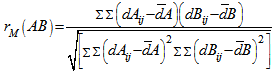 | (1) |
 denotes the double summation over and
  which ranges from one to n and
  by symmetry of
  and
and  , and
, and  and
and  are means of distances derived from the
  and
and  raw data respectively.The testing procedure is given as stated by[3]:1. Considering two symmetric resemblance matrices (similarities)
  and
and  , of size (
 ), whose rows and columns correspond to the same set of objects. Compute the Pearson correlation (alternatively, the spearman correlation) between the corresponding objects of the upper-triangular (or lower-triangular) portions of these matrices, obtaining the mantel correlation (often called the standardized Mantel statistic)
  , which will be used as the reference value in test.2. Permute at random the rows and corresponding columns of one of the matrices, say
  , obtaining a permuted matrix
  . This procedure is called ‘matrix permutation’.3. Compute the standardized Mantel statistic
  between matrices
  and
and  , obtaining a value
  of the test statistic under permutation.4. Repeat steps 2 and 3 a large number of times to obtain the distribution of
  under permutation; then, add the reference value
  to the distribution.5. For a one – tailed test involving the upper tail (i.e., H 1+: distances in matrices
  and B are positively correlated), calculate the probability (p – value) as the proportion of values
  greater than or equal to
  . For a test in the lower tail, the probability is the proportion of values
  smaller than or equal to
  .Note that for symmetric distance matrices, only the upper (or lower) triangular portions are used in the calculations while for non symmetric matrices, the upper and lower triangular portions are included. The main diagonal elements need not be included in the calculation, but their inclusion does not change the p- value of the test statistic.
2.2. Source of Data
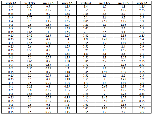
- The source of data used for this study is secondary data obtained from the records department of Ekeukwu Farms Anambra state – Nigeria for a period of eight weeks, weight measured in kg. Where we were informed that sixty broiler birds were divided into two groups, one group A was feed with the first feed while group B was feed with another type of feed. The weights of the birds were recorded weekly for the period of eight weeks in kilogram.
2.3. Data Presentation
3. Analysis
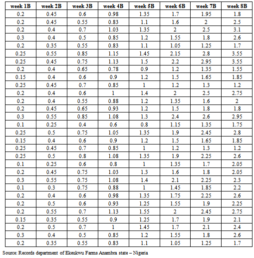
- Inputting the data in Table 1 and Table 2 on R 2.13.0 command window;[10], where week1A, week2A, week3A, week4A, week5A, week6A, week7A and week8A are objects of matrix A; that is, broiler birds fed with feed A while week1B, week2B, week3B, week4B, week5B, week6B, week7B and week8B are objects of matrix B; that is, broiler birds fed with feed B. R> week1A=c(0.30, 0.20, 0.25, 0.30, 0.40, 0.20, 0.30, 0.35, 0.15, 0.25, 0.20, 0.25, 0.25, 0.25, 0.20, 0.25, 0.30, 0.20, 0.15, 0.15, 0.25,0.20, 0.10, 0.20, 0.20, 0.25, 0.05, 0.20, 0.15, 0.15)R > week2A=c(0.55, 0.60, 0.60, 0.75, 0.80, 0.60, 0.60, 0.65, 0.45, 0.65, 0.55, 0.60, 0.55, 0.50, 0.50, 0.65, 0.65, 0.55, 0.50, 0.50, 0.50, 0.50, 0.25, 0.60, 0.65, 0.50, 0.30, 0.60, 0.50, 0.50)R > week3A=c(0.90, 0.85, 0.90, 1.10, 1.15, 0.85, 0.85, 1.00, 0.65, 0.90, 0.85, 0.90, 0.80, 0.90, 0.75, 0.90, 0.85, 0.85, 0.90, 0.75, 0.80, 0.75, 0.30, 0.85, 0.85, 0.75, 0.35, 0.80, 0.90, 0.75)R > week4A=c(1.15, 1.05, 1.38, 1.60, 1.55, 1.05, 1.25, 1.55, 1.05, 1.40, 1.20, 1.25, 1.10, 1.35, 1.15, 1.38, 1.30, 1.20, 1.18, 1.15, 1.18, 1.03, 0.35, 1.05, 1.20, 0.95, 0.45, 1.20, 1.18, 1.15)R > week5Aa=c(1.40, 1.55, 1.85, 2.10, 2.05, 1.25, 1.65, 2.10, 1.45, 1.90, 1.55, 1.55, 1.25, 1.80, 1.55, 1.85, 1.75, 1.55, 1.45, 1.55, 1.55, 1.30, 0.50, 1.55, 1.55, 1.15, 0.50, 1.65, 1.45, 1.55)R > week6A=c(1.70, 2.00, 2.30, 2.60, 2.55, 1.50, 2.00, 2.50, 1.90, 2.45, 1.70, 2.00, 1.50, 2.10, 2.10, 2.20, 2.00, 1.80, 1.95, 1.90, 2.00, 1.80, 0.65, 2.00, 2.00, 1.45, 0.55, 2.00, 1.95, 1.90)R > week7A=c(1.80, 2.25, 2.70, 3.30, 3.15, 1.95, 2.30, 3.10, 2.35, 2.85, 1.95, 2.40, 1.55, 2.50, 2.55, 2.60, 2.55, 2.10, 2.35, 2.20, 2.45, 1.95, 1.15, 2.45, 2.25, 1.75, 0.60, 2.35, 2.35, 2.20)R > week8A=c(1.65, 2.65, 3.10, 3.50, 3.30, 2.30,2.50, 3.50, 2.65, 3.40, 2.20, 2.90, 1.70, 3.10, 2.80, 2.85, 2.75, 2.10, 2.65, 2.50, 2.70, 2.50, 1.60, 2.70, 2.65, 1.80, 0.75, 2.70, 2.65, 2.65)R > week1B=c(0.20, 0.20, 0.20, 0.30, 0.20, 0.25, 0.25, 0.20, 0.15, 0.25, 0.20, 0.20, 0.20, 0.30, 0.10, 0.25, 0.15, 0.25, 0.25, 0.10, 0.20, 0.30, 0.10, 0.20, 0.20, 0.20, 0.15, 0.20, 0.30, 0.20)R > week2B=c(0.45, 0.45, 0.40, 0.40, 0.35, 0.55, 0.45, 0.40, 0.40, 0.45, 0.40, 0.40, 0.45, 0.55, 0.25, 0.50, 0.40, 0.45, 0.50, 0.25, 0.45, 0.55, 0.30, 0.40, 0.50, 0.55, 0.35, 0.50, 0.40, 0.35)R > week3B=c(0.60, 0.55, 0.70, 0.50, 0.55, 0.85, 0.75, 0.65, 0.60, 0.70, 0.60, 0.55, 0.65, 0.85, 0.40, 0.75, 0.60, 0.70, 0.80, 0.60, 0.75, 0.75, 0.75, 0.60, 0.60, 0.70, 0.55, 0.70, 0.50, 0.55)R > week4B=c(0.98, 0.83, 1.03, 0.85, 0.83, 1.15, 1.13, 0.78, 0.90, 0.85, 1.00, 0.88, 0.93, 1.08, 0.60, 1.05, 0.90, 0.85, 1.05, 0.80, 1.03, 1.08, 0.88, 0.98, 0.93, 1.13, 0.90, 1.08, 0.85, 0.83)R > week5B=c(1.35, 1.10, 1.35, 1.20, 1.10, 1.45, 1.50, 0.90, 1.20, 1.00, 1.40, 1.20, 1.20, 1.30, 0.80, 1.35, 1.20, 1.00, 1.35, 1.00, 1.30, 1.40, 1.00, 1.35, 1.25, 1.55, 1.25, 1.45, 1.20, 1.10)R > week6B=c(1.70, 1.60, 2.00, 1.55, 1.05, 2.15, 2.20, 1.20, 1.50, 1.20, 2.00, 1.35, 1.50, 2.40, 1.15, 1.90, 1.00, 1.20, 1.90, 1.35, 1.60, 2.10, 1.45, 1.75, 1.55, 2.00, 1.70, 1.70, 1.55, 1.05)R > week7B=c(1.95, 2.00, 2.50, 1.80, 1.25, 2.80, 2.95, 1.35, 1.65, 1.30, 2.50, 1.60, 1.80, 2.60, 1.35, 2.45, 1.65, 1.30, 2.35, 1.70, 1.80, 2.25, 1.85, 2.25, 1.90, 2.45, 1.90, 2.10, 1.80, 1.20)R > week8B=c(1.80, 2.50, 3.10, 2.60, 1.70, 3.55, 3.50, 1.55, 1.85, 1.20, 2.75, 2.00, 1.80, 2.95, 1.75, 2.80, 1.85, 0.20, 2.60, 2.05, 2.05, 2.30, 2.20, 2.60, 2.25, 2.75, 2.10, 2.40, 2.60, 1.70)R > A <-matrix(c(week1A, week2A, week3A, week4A, week5A, week6A, week7A, week8A), nrow = 8, byrow = TRUE)R > B <-matrix(c(week1A, week2A, week3A, week4A, week5A, week6A, week7A, week8A), nrow = 8, byrow = TRUE)It should be of interest to note that the class distance of matrices A and B as defined above are based on canonical measure (method = 1), labelled as DA and DB respectively. R > DA <-dist.quant(A, method = 1)R > DB<-dist.quant(B, method = 1)
|
 Similarly, below is the elements of distance matrices DB which contains objects of matrix B on a class distances based on the canonical measure (method =1). Where the result displayed by DB expressed that the distance between week1B and week1B; week2B and week2B; week3B and week3B; week4B and week4B; week5B and week5B; week6B and week6B; week7B and week7B; week8B and week8B , is 1, distance between wee1B and week2B is 1.235921; week1B and week3B is 2.463230; week2B and week3B is 1.282576; week1B and week4B is 4.046146; week2B and week4B is 2.838450; week3B and week4B is 1.658855; week1B and week5B is 5.650442; week2B and week5B is 4.446909; week3B and week5B is 3.294693; week4B and week5B is 1.636398; week1B and week6B is7.918017; week2B and week6B is 6.729970; week3B and week6B is 5.561250; week4B and week6B is 3.981495; week5B and week6B is 2.521408; ... ; week7B and week8B is 168.817135.
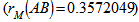
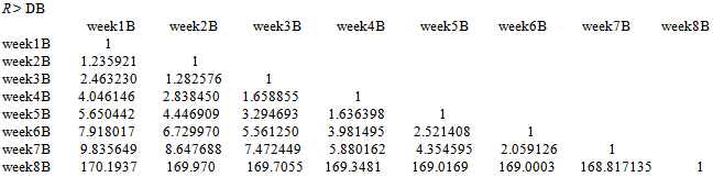 The mantel.rtest function was used to perform the mantel test for 10000 permutations, where “nrept” represents the number of permutations;R > mantel.rtest(DA, DB, nrepet = 10000)Monte-Carlo testObservation: 0.3572049 Call: mantel.rtest(m1 = DA, m2 = DB, nrepet = 10000)Based on 10000 replicatesSimulated p-value: 0.00019998
4. Discussion
- From the result obtained above, it was observed that there exist a week positive resemblance between the weekly weight of Group A broiler birds and Group B broiler birds with an association of 35.72%
 which on the mantel.rtest function result was indicated as observation = 0.3572049 and a P-value of 0.0002 which fall’s on the rejection region with a significance level of 5% (α = 0.05); this implies that there is presence of statistical significance on the weekly weight of the two groups of broiler birds. Since, there exist significance difference between the weekly weights of the two groups of broiler birds; it should be appreciated to express graphically the average weekly behaviour in weight of the two groups of broiler birds. Hence, it was observed from Figure 1 that the average weekly weight of broiler birds fed with feed A was found to weigh more than broiler birds fed with feed B for the observed period of eight weeks.
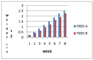 | Figure 1. Distribution of the average weekly weight of birds feed with feed A and feed B |
5. Conclusions
- From the discussion, it was denoted that there exists a linear weak positive resemblance between the weight of Group A broiler birds and Group B broiler birds and the presence of statistical significance. This result implies that the weekly weights of the two Groups of broiler birds are not statistically equal. It was equally observed that across the observed weeks that broiler birds fed with feed A weigh more than broiler birds fed with feed B as was expressed in Figure 1. This implies that broilers fed with feed A was able to perform better in weight across the observable weeks than broilers fed with feed B. Hence, the broiler production manager is best advised to keep up with feed A in other to obtain a better production of broiler birds and profitability.
Appendix A
- Illustrative Manual Solution of the MethodologyFrom Appendix A, we shall unfold the lower objects of matrices DA and DB into column A and B in Table 3 below:
|
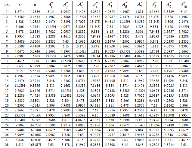
 are the various permutations of the vector A.Using the formula labelled Equation 1, we shall obtain the following measure to form the distribution under 10 permutations as given;
 and the measures below forms
  (the distribution under permutation) for 10 permutations;
 For a one – tailed test involving the upper tail, we calculate the probability as the proportion of values
  greater than or equal to
  . Since the number of
  (the reference value) is given as p-value= 0/10= 0.00. We should understand that as the number of permutation increases to 10,000 to 50,000 permutations the distribution under permutation stables and the dist.quant method use is method 1 which is the canonical measure.