1. Introduction

The eddy covariance technique is generally used to estimate turbulence fluxes of mass and energy to and from surfaces. A difficult but important issue remains to quantify estimates of the uncertainty of the reported flux values. These fluxes are in fact complex processes, and the estimates result from various measurements and calculations as well as numerous explicit and implicit assumptions[4,23]. Hence, documenting the absolute accuracy of these values is somewhat problematic. However, one simple measure of internal consistency is to check for conservation of energy. So the sum of the turbulence fluxes of sensible and latent heat should balance the available energy[9]. The surface energy balance may be written as in (1).

(1)

Where R_n is net radiation, G is soil heat flux, H is the sensible heat flux and LE is latent heat flux. In a perfect world, measurements would be perfect and the closure value would be close to 1.

The source area of a turbulent flux defines the spatial context of the measurement. It is something akin to the “field of view” of the measurement of surface atmosphere exchange. When turbulent flux sensors are deployed, the objective is usually to measure signals that reflect the influence of the underlying surface on the turbulent exchange. The measured signal depends on which part of the surface has the strongest influence on the sensor, and thus on the location and size of its footprint[17]. The footprint size can be considered like a representative area of the sensor detector. Generally the footprint can be represented like a distance from the tower (where sensors detector are located) upwind the preferential direction of the wind velocity. Many models are available to calculate the footprint dimension; for example the Lagrangian, Eulerian and LES (Large Eddy Simulation) models are very complicated but they try to represent the conditions of the atmospheric turbulence in a realistic way[5,11,12,14,15,21]. One of the problems of these models is the computational cost required to solve equations. A simple model based on the combination of Lagrangian stochastic model and dimensional analysis is represented by the Hsieh’s hybrid model[10]. The advantage of this model is that it can be applied in neutral, stable and unstable conditions and compared with Gash’s Eulerian model[8] and Thomson’s Lagrangian model[20] results, produces a correct assess of the footprint size.

There are several reasons because the balance closure value is not perfectly 1[7], but two principal problems are: the dimension of source area for eddy fluxes measurements and stability conditions of the atmosphere. The objective of this work is to show how the energy balance closure changes using only flux measurements with a source area equal to the field size. Moreover, it is shown how the slope values of the linear regression for energy balance closure and the footprint dimension changes according to the different stability conditions of the atmosphere (unstable, neutral e stable conditions).

2. Theoretical Background

2.1. Eddy Covariance Technique

The turbulence of the air flow can be described, using the Reynold’s hypothesis, subdividing wind speed and the scalar quantities in a mean component and in a fluctuant component (2).

(2)

The U,V,W are the instantaneous three-dimensional components of the wind speed, T is the scalar temperature and q is the scalar concentration of vapour in air. , , , and represents the mean components and the u’,v’,w’,T’ and q’ represents the fluctuant components. It is important to remark that these components are a function of the spatial position (x,y,z) and time (t).

The eddy covariance method determines the surface fluxes as the sum of turbulent eddy-fluxes, measured above the surface, and the flux divergence between the surface and the eddy covariance measurement level[2]. The basic equations to estimate latent and sensible heat fluxes, (3) and (4), are comparatively simple.

(3)

(4)

Where is the vaporization latent heat, the air density and the covariance between vertical wind velocity component and scalar concentration of vapor in the air. C_p is the specific heat at constant pressure and is the covariance between vertical wind velocity component and scalar temperature.

The covariance of the vertical wind velocity and scalar quantities can be determined by (5):

(5)

Where represents a generic scalar quantity and N the total number of data.

The energy balance closure can be written as (6):

(6)

R_n and G can be calculated using respectively equation (7) and (8).

(7)

(8)

The net radiation in the atmosphere is divided into shortwave radiation and long wave radiations. The net radiation is the sum of the shortwave down welling radiation mainly from the sun (R_{s_i}), the long wave dowelling infrared radiation emitted by clods, aerosol and gases (R_{l_i}), the shortwave up-welling reflected radiation (R_{s_o}) and the long wave up-welling infrared radiation (R_{l_o})[6].

The ground heat flux is based on molecular heat transfer and is proportional to the temperature gradient in the soil and the thermal molecular conductivity a_G.

The a_G values in function of the different types of ground surface can be found in[18]. On summer days, the ground heat is about 50-100 Wm^-2[6].

LE, H, G and R_n have a totally different representative source areas. LE and H are turbulent fluxes and their representative source area is defined by the footprint size[10]. It depends to the turbulent characteristics of the atmosphere and many other variables for example roughness, wind velocity, measurement height and so on[6]. Its value goes from some meters square to hectares. For R_n the representative source area is characterized by the radiometer field of view and it depends, in particular way, on the measurement height. The net radiometer is located on the tower at the height of about 4 meters (see Section 3) and its field of view can be considered of about 50m² (for an angle of 45°). Ground heat flux (G) is usually very small respect to the other energy fluxes, ranging from 5 to 40 % of net radiation but this flux is the one with the highest uncertainty in its estimate that can reach en error up to 50%[6]. Moreover it is measured with an instrument with the smallest source area that can be up to two orders of magnitude lower than latent and sensible heat fluxes footprints; however, in literature it is assumed that the net radiation and ground heat flux measurements are representative for the total cultivated field[6].

2.2. The Hsieh’s Model

The Hsieh’s model [10] is based on the equation (9).

(9)

x represents the distance from the tower, k is the Von Karman constant and its value is 0.4, D and P are called similarity constants and depend on stability conditions of the atmosphere[10]. z_u is a length scale and z_m represents the height where sensors are installed. F/S₀ is the ratio between the flux measured by the sensors and the flux emitted by the total field. S₀ quantity is not known but it is not important because the ratio is always confined from 0 to 1[10]. L is the Monin - Obukov length[3] and can be calculated by equation (10).

(10)

Where u_* is the friction velocity (11), is the mean air temperature, g is the gravity constant and k the Von Karman constant.

(11)

Where and are the covariance between vertical velocity component and planar (longitudinal and transversal) components of the wind, and z_u is defined by (12) where z₀ represents the surface roughness.

(12)

In growing period it is necessary to change the measurement height z_m in (z_m-d) where d is called displacement and it is about 2/3 of h_v[6] where h_v is the vegetation height. The roughness is calculated by the approximate relation[6] (13).

(13)

3. Study Sites and Instruments

Experimental data were obtained by two micrometeorological stations utilized to measure evapotranspiration fluxes in maize fields, one in Landriano (PV) (45.19 N, 9.16 E, 87 m a.s.l) and another one in Livraga (LO) (45.11 N, 9.34 E, 60 m a.s.l) (Figure 1). The distance between the stations is about 100 Km and they are located at the Po valley.

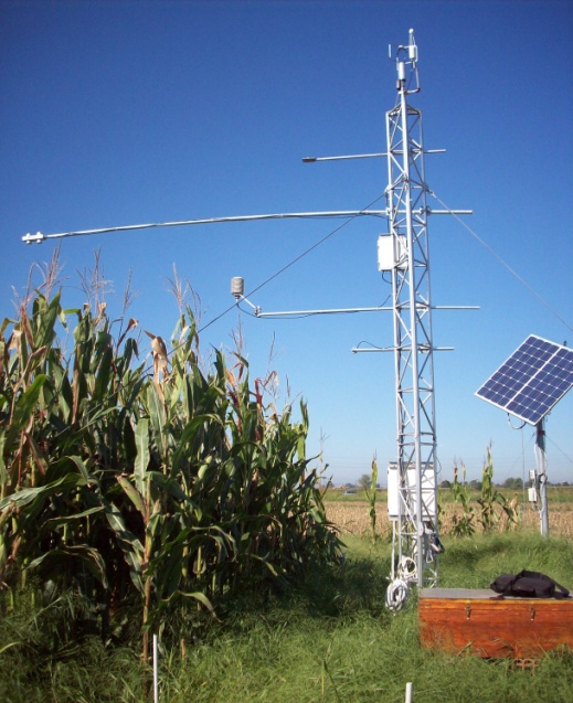Figure 1. Eddy covariance tower at Livraga (LO).

Both data stations are acquired by a Campbell Scientific data logger (CR 5000) and stored each 30 minutes. The stations are equipped with the following sensors: one 3D sonic anemometer (Young 81000 by Young), that measures air temperature and the three components of wind speed and is positioned at 5m height; a gas analyzer (LICOR 7500 by LICOR) for the measurement of air humidity, working with the anemometer at a frequency of 10Hz, is also positioned at 5m height; a radiometer (CNR1 by Kipp & Zonen), which measures the four components of net radiation, is positioned at 4m height; two thermocouples (by ELSI) and a heat flux plate (HFP01 by Hukseflux) for the measurement of soil ground heat flux positioned respectively at 6-10 cm and 8 cm; humidity probes (CS616 by Campbell Scientific) for measurement of the volumetric soil moisture at different depths; a pluviometer (AGR100 by Campbell Scientific) at 1.5m height.

Data which are used in this work were collected during the year 2010, from 1^th June (152^th Julian day) to 10^th October (283^th Julian day) for Landriano site and from 25^th May (145^th Julian day) to 10^th September (253^th Julian day) for Livraga site.

Energy fluxes have been corrected applying Webb correction for density fluctuations[22] and the correction for buoyancy flux due to sonic temperature measurements [13].Tilt correction has been applied to take into account that the assumption of a negligible mean vertical velocity is not always verified[19]. Frequency response correction has been applied for the attenuation of eddy covariance fluxes due to sensor response, path-length averaging, sensor separation, signal processing, and flux averaging period[16]. The data during rainfall period were discarded.

The database, after these corrections, is composed of 4163 and for 4507 half hourly data respectively for Landriano and Livraga.

Figure 2. a. Landriano field, b. Livraga field. Subdivision in sectors.

4. Method

The objective of this work is to understand the influence of the representative source area for eddy covariance measurements on energy balance closure.

The first step was to subdivide Landriano and Livraga fields in four different sectors along geographic directions (Figure 2a and b) so that the data were subdivided in four classes of 90 degree each depending on wind direction.

For each sector it was definite a radius of a source area which is included at least 95% into the field. In Table 1 the radius value taken for each sector is shown.

Table 1. Sectors dimension Radius (m) Sector Landriano site Livraga site I 160 195 II 100 90 III 120 120 IV 200 165

For each measurement of latent and sensible heat fluxes was associated the corresponding footprint size using the relation (9) (assuming that F/S₀ value is equal to 0.8), the prevalent wind direction and its sector. It was assumed a value of F/S₀ equal to 80% because it represents, in according to the results shown in[10], a typical value over which the footprint shape does not change significantly. The data of latent or sensible heat which had a corresponding source area larger than their respective radius, were deleted.

The energy balance was calculated using equation (6) where LE, H, R_n and G were determined by (3), (4), (7) and (8). One main objective of this work is to show how the energy balance closure was influenced by stability conditions of the atmosphere. To define the stability conditions it was taken the stability parameter (z_u/L). If z_u/L < -0.04 the atmosphere is in unstable conditions; for z_u/L > 0.04 there are stable conditions and for -0.04 < z_u/L < 0.04 the atmosphere is in neutral conditions. This classification is, also, important to define the value of D and P [10] in (9). For these different atmospheric situations the slope values of linear regression (m) and linear correlation coefficients (R²) for the energy balance closure were calculated. Moreover, it was studied the energy balance closure for different sectors depending on wind direction. For Landriano and Livraga site LE, H, R_n and G were collected in four groups: from 0° to 90°, from 90° to 180°, from 180° to 270°, from 270° to 360° and for each group the slope of the energy balance closure was calculated. At the same time, it was made a study about source area size and its variability for different atmospheric conditions. A frequency analysis on footprint size was made during instable and neutral conditions because the eddy covariance station works only if there is turbulence into the atmospheric boundary layer[6] and it is guaranteed only in convective (unstable) or neutral conditions[6], instead, in stable conditions the turbulence is formed by eddies which have small dimension (some centimetres) and are originated by the mechanical forces of the wind shear[24]. In these cases the atmosphere is quite similar to a laminar structure. For each sector the footprint values were subdivided in twenty classes and subsequently the number of footprint values which fallen in each class was calculated. It was also shown the percentage of data which had to be deleted because the footprint size was larger than field dimension.

5. Results and Discussion

The results show that the slope of the energy balance closure increases slightly if the data without a footprint size compatible with the field dimension were deleted. In Figure 3 and 4 are shown the energy balance closure respectively for Landriano and Livraga site. In Figure 3a and 4a are represented the energy balance closure for all data set, while in Figure 3b and 4b the energy balance closure is calculated using only the footprint compatible data. For Landriano site, the slope of the linear regression has a slight improvement of about 0.40% and for the linear correlation coefficient of about 3.8%. For Livraga site, the difference in slope is 0.33% and in R² is equal to 4.24%

Figure 3. Landriano site. a. energy balance closure with all data. b. energy balance closure using the data with a footprint compatible with field dimension.

Considering only the data which have a footprint size compatible with the fields dimension, for Landriano site, the number of data changes from 4163 to 2329, which represents about 55% over total data set. For Livraga site, the number of data changes from 4507 to 2401 which represents about 53% over total data set.

Figure 4. Livraga site. a. energy balance closure with all data. b. energy balance closure using the data with a footprint compatible with field dimension.

In the Po Valley the geometric structure of the fields have a polygonal shape and there are irrigation ditches around them. Landriano and Livraga fields are surrounded by other maize fields and it is probable that the slight improvement of the linear regression slopes is caused by the quite similar evapotranspiration among the fields. Moreover, the fields dimensions are smaller than those in USA country[1]. In fact Landriano and Livraga fields are about 10 hectare large. For example in Boardman, OR (USA), the fields have a circular shape and they are surrounded by the desert. In these cases the spatial variability of surface fluxes is very big, in fact in [1] is shown that the variation of measured latent heat flux densities across a potato field from discontinuity point (desert-field) to the centre of the field is about 60%.

The stability conditions of the atmosphere play an important role on the energy balance closure improvement. In Table 2 and 3 the values of m and R² are shown for different stability conditions of the atmosphere (stable, neutral and unstable conditions). The value of m shown in Table 2 and III confirmed that in unstable and neutral conditions the heat fluxes measured by the eddy tower are correct while in stable conditions the heat fluxes are incorrect because the turbulence structure into the atmospheric boundary layer is not well definite[24].

So, in additions to the flux corrections indicated in Section 2 the flux data measured in stable conditions have to be deleted; in these cases it is nonsense to talk about representative source area for turbulent heat fluxes. For this reason in Table 2 and 3 the value of the slope and R² in “fluxes with footprint” are not indicated.

The footprint dimension is a main feature which has to be used to choose the correct turbulent flux data. In unstable and neutral conditions the representative source area for latent and sensible heat fluxes can be larger than field dimension. In these cases the flux data have to be deleted. The effect of the data removal is shown in Table 2 and 3 with reference to “Fluxes with footprint” and “N° data with footprint”.

Table 2. Landriano site. Slope values of the linear regression (m) and linear correlation coefficient (R2) for different stability conditions of the atmosphere for all data set and for only the data which have a footprint size compatible with field dimension. Total fluxes Fluxes with footprint N° data % of data N° data with footprint % data with footprint m R2 m R2 Unstable conditions 0.6453 0.9045 0.6467 0.9097 1980 47.6 1840 44.2 Neutral conditions 0.6552 0.9035 0.6609 0.9478 977 23.5 477 11.5 Stable conditions 0.1415 0.0744 1206 29.0 Total data 0.6433 0.8715 0.6473 0.9095 4163 100.0 2329 55.9

Table 3. Livraga site. Slope values of the linear regression (m) and linear correlation coefficient (R2) for different stability conditions of the atmosphere for all data set and for only the data which have a footprint size compatible with field dimension. Total fluxes Fluxes with footprint N° data % of data N° data with footprint % data with footprint m R2 m R2 Unstable conditions 0.6790 0.8750 0.6770 0.8820 1725 38.3 1611 35.7 Neutral conditions 0.7050 0.8220 0.6980 0.8420 1276 28.3 893 19.8 Stable conditions 0.0290 0.0070 1386 30.8 Total data 0.6760 0.8070 0.6790 0.8490 4507 100.0 2401 53.3

The slight improvement on m and R² in function of the different stability conditions of the atmosphere (unstable and neutral) is shown in Table 4. While in Landriano site in unstable and neutral conditions the slope of the linear regression for the energy balance closure (from “Total fluxes” to “Fluxes with footprint”) increase its value, in Livraga site it decreases. However, using the total data set which is also composed by data measured in stable conditions, the slight improvement on m value for Livraga site is guaranteed how shown in Table 2 and 3. The dispersion of the points around the linear regression curve is minimized; in fact the value of R² increases in Landriano and Livraga site for unstable and neutral conditions.

Table 4. Energy balance closure improvement on m and R2 for different conditions of the atmosphere, for Landriano and Livraga site. Unstable conditions Neutral conditions Landriano Improvement on m (%) 0.14 0.57 Improvement on R2 (%) 0.52 4.43 Livraga Improvement on m (%) -0.20 -0.70 Improvement on R2 (%) 0.70 2.00

5.1. Energy Balance Closure for Field Sectors

In Figure 5 and 6 the energy balance closure and the footprint size for the different field sectors as a function of the wind directions are shown. In Figure 5A and 6A the energy balance closure taking into account all data set is represented, while in Figure 5B and 6B the energy balance closure is made using only the data with a footprint length compatible with the field dimension. The energy balance closure characterization for different sectors is necessary to understand how each sector field takes part on total energy balance closure. In fact in some cases it is present an m value improvement (sectors I, II and IV for Landriano, and sectors I, III and IV for Livraga) but in other cases the m value decrease (sector III for Landriano and sector II for Livraga).

In Table 5 the percentages of improvement of the slope of linear regression and R² for the data which have a footprint size included into the field are represented. In general in Landriano and Livraga sites for almost all the sectors a slight improvement in both m and R² values is presented. In Figure 5 and 6 (C and D) the footprint sizes for different classes subdivided in unstable and neutral conditions of the atmosphere are represented. During convective conditions the source area lengths are distributed over all the footprint classes, while in neutral conditions only some classes have the most part of the footprint values.

Figure 5. Landriano site. A. Energy balance closure with all data. B. Energy balance closure using the data which have a footprint size less than field dimension. C. Footprint length for unstable conditions of the atmosphere. D. Footprint length for neutral conditions of the atmosphere.

Figure 6. Livraga site. A. Energy balance closure with all data. B. Energy balance closure using the data which have a footprint size less than field dimension. C. Footprint length for unstable conditions of the atmosphere. D. Footprint length for neutral conditions of the atmosphere.

Table 5. Energy balance closure improvement on m and R2 for each sector, for Landriano and Livraga site. I SEC. II SEC. IIISEC. IVSEC. Landriano Improvement on m (%) 3.23 0.37 -0.040 0.69 Improvement on R2 (%) 6.50 1.62 0.44 1.31 Livraga Improvement on m (%) 0.83 -0.75 0.36 0.68 Improvment on R2 (%) 1.99 4.87 1.79 1.3

Table 6. Footprint data which have a length less than the field dimension I SEC. II SEC. IIISEC. IVSEC. Landriano Unstable conditions (%) 99.10 84.80 88.60 100.00 Neutral conditions (%) 55.60 0.00 0.00 40.40 Livraga Unstable conditions (%) 99.70 73.40 90.00 96.70 Neutral conditions (%) 79.20 0.00 54.60 76.70

In Table 6 the percentage of the footprint data with a length less than the radius is shown. Only during the convective conditions, the footprint size is almost compatible with the field dimension and the percentage of data which can be used is >80%. Instead, in some cases where there are neutral conditions of the atmosphere the footprint size is completely larger than field dimension and the flux data can not be used.

6. Conclusions

In this work the effect of the source area of eddy covariance measurements on energy balance closure for maize fields in Po Valley has been shown. The energy balance was evaluated for different conditions of the atmosphere and to understand their effects on the closure, the slope of the linear regression (m) and the linear correlation coefficient (R²) were calculated. The results show that the eddy covariance stations works only in unstable and neutral conditions. In stable conditions the atmospheric boundary layer structure is quite laminar and the turbulent heat fluxes measured by the eddy tower are uncorrected. During neutral conditions, a lot of data have to be deleted because the turbulent fluxes source representative area exceeds the field dimension. In Landriano and Livraga site the effect of the representative source area for eddy fluxes leads to a slight improvement into the energy balance closure, instead, the stability conditions of the atmosphere play a fundamental role for the determination of the slope of the linear regression curve. The study on the representative source area for eddy covariance measurements is important to understand if the station position into the field is correct, the energy balance closure makes for different sector in function of the wind directions shows that in Landriano and Livraga sites the eddy covariance towers are located correctly and the latent and sensible heat measured are representative of the maize fields.

ACKNOWLEDGES

This work was funded in the framework of the ACQWA EU/FP7 project (grant number 212250) “Assessing Climate impacts on the Quantity and quality of WAter”, the framework of the ACCA project funded by Regione Lombardia “Misura e modellazione matematica dei flussi di ACqua e CArbonio negli agro-ecosistemi a mais” and PREGI (Previsione meteo idrologica per la gestione irrigua) founded by Regione Lombardia. The authors thank the University of Milan – Dipartimento di Idraulica Agraria for the collaboration given in managing Landriano eddy covariance station.